What pretraining is, and the budget first
A base model learns a distribution of text by minimising next-token cross-entropy, usually over a mixture of documents packed into fixed-length sequences:
Here |\mathcal D| counts predicted tokens. The tokens provide their own targets; the text can contain tasks or instructions, but the objective does not require separate human labels. Loss is in nats per token and its exponential is perplexity (Module 07). Pretraining produces the base; Module 09 adds instruction and preference training.
Decide before the expensive run
Fix the tokenizer, model shape, data policy and schedule before launch. Changing them later can require retokenisation, weight migration or a revised training phase. Small ablations should settle uncertain choices before the long run pays for them. Later mixture changes and batch ramps remain possible if documented.
| Decision | Evidence to obtain | Section |
|---|---|---|
| Model size and training tokens | Compute accounting and scaling fits | 1 |
| Sources, filters, deduplication and contamination | Audited removals and proxy-model ablations | 2, 3 |
| Mixture, tokenizer and packing | Source exposures and compression tests | 4 |
| Shape and optimiser | Parameter counts and small sweeps | 5, 6 |
| Precision and stabilisers | Mechanism-specific diagnostics | 7 |
| Memory and parallel layout | Arithmetic followed by measurement | 8–10 |
| Recovery and evaluation | Failure logs, held-out losses and task uncertainty | 11, 12 |
| Small runs and domain adaptation | Baselines and a declared acceptance gate | 13, 14 |
The pretraining pipeline, with section references: sources, extraction, language identification, filters, deduplication, decontamination, mixture, tokenizer, packed shards, training, checkpoints, evaluation and the base model. Short-run evaluation informs data and recipe decisions before the main run.
The running case study
The hypothetical engineering team from Module 07 adopts a bilingual English–Chinese model to draft and check safety-case arguments for a reactor vessel’s pressure-relief system. It has 36 layers, width 4,096, 32 query/8 KV heads of dimension 128, SwiGLU width 15,360, vocabulary 152,064, untied embeddings, RMSNorm and no biases. Section 5 counts exactly 9,550,729,216 parameters. Arithmetic uses this count; the quick table rounds it to 9.5B, about 0.5% low. It is a worked scenario, not a released product or an actual training plan.
Use it first to understand how such a base could be made: 2T tokens, context 8,192, on 80 H100s. The team adopts a released checkpoint rather than running that plan. Its own possible run is continued pretraining on 1.8B domain tokens plus 0.2B general replay, accepted only after the baseline and gate in Section 14. Module 09 post-trains the kept checkpoint, or the instruct release if adaptation fails; Module 10 serves the result.
Use one FLOP convention
Module 06 derives the count. A matrix weight costs approximately two forward FLOPs per token; backward costs twice forward. The input embedding is a lookup, so the untied model has N_{\text{matmul}}=N-Vd. Causal attention averages 2LdT forward FLOPs per token over a length-T sequence. The architecture-aware training estimate is
Memory counts all N. Chinchilla’s published fit uses its own budget C_6=6ND, without the explicit attention term. Keep that convention for its iso-FLOP curves and payback calculations; elsewhere label 6ND as a shortcut. These are model arithmetic estimates, excluding communication and most elementwise operations. Some papers charge full-square attention: PaLM’s utilisation count uses 6N+12LTd. A utilisation figure must state its convention.
The input table has 152064(4096)=622854144 parameters, hence N_{\text{matmul}}=8927875072. At context 8,192:
Attention adds 13.5% to the weight term. The shortcut 6N=57.30 billion is about 7% high on weights and 6% low overall. At context 131,072, attention is sixteen times larger and total cost per token is about 2.8 times the 8k charge.
Convert compute into elapsed time
For sustained per-device rate r, GPU-hours are C/(3600r); divide again by GPU count for elapsed hours. Model FLOPs utilisation (MFU) divides useful model FLOP/s by the hardware peak at the precision used. Hardware FLOPs utilisation (HFU) also counts recomputation, so activation checkpointing can raise HFU without improving useful-token throughput.
The series assumes an H100 SXM dense bf16 peak of 989 TFLOP/s and sustained r=4\times10^{14} FLOP/s, approximately 40% MFU. The exact product 0.40(989) is 395.6 TFLOP/s; use it when the text or widget says exact peak. Sparsity-enhanced peak figures do not apply to dense training. These are planning assumptions; realised throughput, downtime and the chosen layout determine calendar time.
Use 6ND, rounded 9.5B parameters and r=4\times10^{14} FLOP/s throughout this table. These rows are hypothetical comparisons, not historical run records.
| Run | Shortcut FLOPs | GPU-hours | Elapsed time |
|---|---|---|---|
| 9.5B on 190B tokens | 1.083\times10^{22} | 7,521 | 19.6 days on 16 GPUs |
| 9.5B on 2T | 1.14\times10^{23} | 79,167 | 41.2 days on 80 GPUs |
| 9.5B on 15T | 8.55\times10^{23} | 593,750 | 309.2 days on 80 GPUs |
| 1B on 20B | 1.2\times10^{20} | 83.3 | 20.8 hours on four GPUs |
| 9.5B, continued training on 2B | 1.14\times10^{20} | 79.2 | 9.9 hours on eight GPUs |
The exact shape costs 60{,}815{,}007{,}744(2\times10^{12})= 1.2163\times10^{23} FLOPs. At the rounded sustained rate this is 84,465 GPU-hours, or 44.0 days on 80 GPUs. At exactly 40% of the stated peak it is 85,405 GPU-hours and 44.5 days; at 30% MFU, 59.3 days. At the assumed USD 2.50 per GPU-hour, the rounded-rate plan costs about USD 211,000 in GPU time, excluding ablations, failed runs, storage and staff. The 2B-token continued-training plan costs a thousandth as much at the same context.
Allocate the budget for training and serving
Module 07 derives the Chinchilla allocation. The rounded published parametric fit is
Its constants belong to a particular corpus/tokenizer and fitting experiments with 70M–16B parameters and 5B–500B tokens. Twenty tokens per parameter is a heuristic associated with the paper’s other estimation methods; the parametric minimum has a different ratio. Pale curve segments below show extrapolation.
Chinchilla fitted loss at budgets C_6=10^{20},10^{21},10^{22},10^{23}. Circles mark fitted minima and crosses the twenty-token allocation. Diamonds show the 9.55B case model at 190B, 2T and 15T tokens. Curves outside the original parameter/token fitting range are pale; none is a measurement of this case model.
For the exact case shape on 2T tokens, C_6=1.14609\times10^{23}:
| Allocation | Parameters | Tokens | Fitted loss |
|---|---|---|---|
| Case study | 9.551B | 2.000T | 2.00199 |
| Fixed-budget fitted minimum | 15.526B | 1.230T | 1.99848 |
| Twenty tokens per parameter | 30.904B | 0.618T | 2.00537 |
The three losses differ by less than 0.007 nats, while approximate serving arithmetic 2N differs substantially. For an equal-loss comparison, the fitted optimum reaches the case loss at 15.018B parameters on 1.182T tokens, costing C'_6=1.065\times10^{23}. Equating lifetime arithmetic, C_6+2NS=C'_6+2N'S, gives
At the team’s 12M tokens/day that is about 170 years; at ten billion/day it is about 74 days. Producers may serve many users, so their lifetime volume can change the decision. The comparison extrapolates the fit, assumes equal loss means equal quality, and omits attention, quantisation, batching and prices. It does not predict a real deployment’s latency or task score.
Why must a fixed-budget loss minimum be distinguished from an equal-loss serving comparison?
Show answer
A fixed-budget alternative has a different predicted loss. To ask when extra training pays for cheaper serving at equal fitted quality, first solve for an alternative with the same loss, then compare its training and serving charges.
Data I: sources, extraction, language and quality filters
Data quality is the largest lever after scale, and the data pipeline is most of the engineering of a pretraining run. This section and the next two follow the pipeline of Figure 8.1 from raw text to training sequences. Every stage is a rule with a threshold, and every rule removes some text it should have kept, so each is given here with its threshold and what it wrongly removes. Figure 8.3 shows the stages as a funnel.
A filtering funnel drawn as stacked horizontal bars that shrink stage by stage: URL filter, text extraction, language identification, heuristic rules, deduplication and quality classifier. The proportions are illustrative and carry no counts; a side note gives the one published pair used in the text, FineWeb (about 15T tokens) and FineWeb-Edu (about 1.3T). Beside each stage, one example of what it removes: an adult-site URL, a cookie banner, a French page in an English corpus, a navigation bar, a mirrored page, keyword spam.
Sources and the manifest
Common Crawl is the base of nearly every web corpus: a public crawl released as snapshots, roughly monthly, each of billions of pages. A snapshot comes as WARC files, which hold the raw HTTP responses, and WET files, which hold Common Crawl’s own plain-text extraction of them. To the web a corpus adds code repositories, books, academic papers, reference works and forums. For a bilingual model like the case study’s it adds the Chinese web, Chinese books and Chinese academic text, in proportion to the use the model is for.
Licensing and consent are unsettled and vary by jurisdiction. Opt-outs in robots.txt are honoured at crawl time. The corpus manifest records, for every component, the source, the snapshot or date, the licence, the filters applied and the token count. It is the minimum record: without it nobody can later say what a model was trained on, or rebuild the corpus without a component that turned out to be bad.
Extraction and encoding
A web page is mostly not prose: navigation, cookie banners, footers, repeated headers. Extractors built for the purpose (trafilatura and its kind) locate the main text in the HTML. Running one on the WARC HTML, rather than taking the WET text, pays: the FineWeb authors trained small models on both and found that this choice alone gave better models.
Encoding repair belongs here too. UTF-8 text mis-decoded as Windows-1252 turns an em dash into
—. This mojibake survives every quality rule below, because the words around it are fine.
Lab 1 flags suspicious patterns in 303 of 5,000 original TinyStories
documents, about 6%. Only 97 pass its simple whole-string repair probe. These are
heuristic flags, not a complete encoding audit; leaving artefacts in training data
can teach a model to reproduce them.
Language identification
A linear classifier over character n-gram features gives each document a score per language; fastText’s language-identification model (Joulin et al. 2017) is the common one. Documents whose top score exceeds a threshold (0.65 in FineWeb’s English pipeline) are kept, in the proportions wanted. Character n-grams work because languages differ in their letter combinations within a few words. The classifier fails on short texts, which have too few n-grams to decide; on code-mixed text such as English–Chinese technical writing, which scores partly for each language and may clear neither threshold; and on closely related languages and scripts.
Heuristic quality filters
The Gopher rules (Rae et al. 2021) are cheap statistics over whitespace-separated words. A document is removed if it breaks any of them:
- fewer than 50 or more than 100,000 words;
- a mean word length outside 3 to 10 characters;
- more than 0.1 hash symbols or ellipses per word;
- more than 90% of lines starting with a bullet, or more than 30% ending with an ellipsis;
- fewer than 80% of words containing an alphabetic character;
- fewer than two of the stop words the, be, to, of, and, that, have, with;
- repetition: more than 30% of lines, or of paragraphs, duplicated; more than 20%, 18% and 16% of characters in the most frequent 2-, 3- and 4-gram; more than 15% (for 5-grams) down to 10% (for 10-grams) of characters in duplicated n-grams.
Each rule targets one kind of junk: the length rule fragments and dumps, the symbol rule tag clouds, the bullet and ellipsis rules lists and teasers, the alphabetic rule tables of numbers, the repetition rules templates and spam. The stop-word rule is the cheapest test for prose.
Document (a) is a maintenance note:
The bearing on the pump shaft ran hot for three days before the alarm. Wear on the outer race had loosened the fit, and the extra play let the shaft vibrate. The maintenance team replaced the bearing and checked the alignment with a dial gauge. They also changed the inspection interval from six months to three, because the vibration log showed the fault had been growing for weeks.
Document (b) is the line Home | About us | Contact | Privacy policy | Login | Cart repeated on 5
lines. Document (c) is BUY NOW!!! $$$ #deal CHEAP #sale watches FREE shipping >>> repeated 8
times on one line. Counting whitespace-separated words, with punctuation left attached:
| Statistic | Limit | (a) | (b) | (c) |
|---|---|---|---|---|
| words | 50 to 100,000 | 68 | 5 × 13 = 65 | 8 × 10 = 80 |
| mean word length | 3 to 10 | 4.65 | 3.46 | 4.90 |
| hash symbols per word | at most 0.1 | 0 | 0 | 16/80 = 0.20, fails |
| words with a letter | at least 80% | 100% | 40/65 = 61.5%, fails | 64/80 = 80% |
| stop words present | at least 2 | 4 (and, the, to, with) | 0, fails | 0, fails |
| duplicated lines | at most 30% | 0 | 4/5 = 80%, fails | none (one line) |
(a) passes every rule. (b) passes the length rules because its 65 “words” include the 25 |
tokens, then fails three: letters, stop words and duplicated lines. (c) fails two, symbols and stop
words, and passes the letter rule at exactly 80%. Both junk pages also break the n-gram
repetition limits, since more than half of their characters lie in duplicated 5-grams against a
limit of 15%; that is how (c), a single line, would be caught even without its hashtags.
Lab 1 applies an explicit subset of these rules to a larger corpus and
records the first failure for each document. Its definitions and first-failure
counts should be inspected before comparing it with a full production filter.
C4’s cleaning (Raffel et al. 2020) is the contrast: it works on lines. It keeps only lines that end in terminal punctuation, drops any page that contains “lorem ipsum” or a curly bracket, and drops pages containing any word from a blocklist of obscene words. The curly-bracket rule was aimed at JavaScript left in web pages; it also removes almost all source code, which is why code needs a pipeline of its own (Exercise 5).
Rules are language-specific. Word-based rules do not apply to Chinese, which has no spaces between words, so whitespace splitting turns a Chinese paragraph into a few very long “words”. A Chinese component needs character-based equivalents (length in characters, the share of Chinese characters, repeated character n-grams) and a Chinese stop-word list of common function words such as 的 and 是.
Model-based quality filters
A small classifier trained to separate reference-quality text from random web text scores every document; the corpus is then thresholded on the score, or sampled with a probability that rises with it. FineWeb-Edu (Penedo et al. 2024) is the documented public example. A large language model rated about 450,000 web pages for educational value on a 0–5 scale; a small classifier on top of an embedding model learned those ratings and then scored all of FineWeb, about 15T tokens. Keeping scores of 3 and above left about 1.3T tokens, and models trained on it did better on knowledge and reasoning benchmarks than models trained on the same number of FineWeb tokens. DCLM (Li et al. 2024) trained a fastText classifier for the same purpose, cheap enough to run over a whole crawl.
1.3\text{T}/15\text{T} = 0.087: the classifier kept about 8.7% of the tokens, one in 11.5. A 2T-token run drawing only on FineWeb-Edu would see each of its tokens 2/1.3 = 1.5 times on average, inside the range where repetition costs little (Section 4); a 15T-token run would see each 11.5 times, far outside it. A strict quality filter trades quantity for quality, and the repetition limit decides how far that trade can go.
The failure is narrowing. The classifier encodes its annotator’s taste (encyclopaedic, formal, English-centric), so text that is valuable but unlike its examples, such as maintenance logs, forum troubleshooting threads, code comments and other languages, scores low and disappears.
Personal data and safety
Regular expressions find e-mail addresses, phone numbers and IP addresses. They are replaced with
placeholder tokens such as <EMAIL> rather than deleted, so that the text stays fluent. Names are
hard to find reliably and are mostly left. Over-matching damages technical text: a version string
such as 10.2.0.1 looks like an IP address.
Safety filtering uses URL blocklists and classifiers, and blunt rules do damage of their own: Dodge et al. (2021) found that C4’s word blocklist disproportionately removed text written by and about minority groups. Removing all harmful text also removes the model’s ability to recognise it, which post-training (Module 09) relies on when it teaches the model to refuse.
Order by cost, and keep the log
Run the cheap filters first (URL blocklists, language identification, heuristic rules) and the expensive ones (model classifiers, near-duplicate detection) on what survives. Record why every document was removed. That log is the debugging record when a later model turns out bad: it is how a team discovers that a filter removed the domain it needed.
Why does the stop-word rule catch spam and navigation pages so cheaply?
Show answer
Natural prose almost always contains at least two of the eight commonest English function words, while menus, lists and keyword spam rarely do. The test is one set intersection over words that are already split.
A quality classifier trained to prefer Wikipedia-like text is applied to maintenance logs. What happens, and what do you do?
Show answer
Most logs score low and are removed, although they are exactly the domain text wanted. A quality classifier encodes a style, so domain components get their own filters, or an exemption from the classifier, and the removal log is checked for what each filter took.
Data II: deduplication and decontamination
The web repeats itself. Pages are mirrored, syndicated, templated and copied from one another, and the same licence text, boilerplate and news story appear thousands of times. Duplicates waste compute, raise memorisation and verbatim regurgitation, and tilt the mixture toward whatever was copied most. Two measurements give the size of the effect. Lee et al. (2022) found that models trained on deduplicated C4 emit memorised text about ten times less often and reach the same or better accuracy in fewer steps. Hernandez et al. (2022) found that repeating 0.1% of the data 100 times degraded an 800M-parameter model to the performance of one half its size, although 90% of the training tokens stayed unique.
Exact duplicates
Normalise each document (lower-case it, collapse whitespace), hash it (SHA-1, or any good 64-bit hash), and keep the first occurrence of each hash. The same pass at line and paragraph level, across documents, strips boilerplate repeated on thousands of pages: cookie notices, footers, licence paragraphs. The fine-grained version works on substrings: a suffix array of the corpus finds every span that occurs more than once, and Lee et al. removed repeated spans of 50 tokens or more.
Near-duplicates and Jaccard similarity
A page with a changed date, a different advertisement or a few edited words hashes differently. To catch near-duplicates, represent each document by its set of shingles, the word n-grams it contains (5-grams here), and measure the overlap of two sets with the Jaccard similarity
Computing J for every pair is hopeless at web scale. MinHash estimates it from short signatures, and banding avoids comparing most pairs at all (Figure 8.4).
MinHash and banding in one picture. Two short documents become their sets of 5-word shingles, drawn as overlapping circles with the intersection shaded and J written beside them. Each set becomes a 128-slot signature, drawn as 16 bands of 8 cells. The bands in which the two signatures agree in all 8 cells are highlighted, which makes the documents a candidate pair, and the pair is then verified with the exact Jaccard similarity.
MinHash, derived
Apply a random permutation \pi to the universe of shingles and record, for each set, its smallest permuted value. Then
The proof is short. Consider the smallest element of \pi(A \cup B). A random permutation favours no element, so it is equally likely to be any of the |A \cup B| elements of the union. If it lies in A \cap B, it is the minimum of both sets and the two minima coincide. If it lies in only one set, it is that set’s minimum, and the other set’s minimum is a different, larger value. So the minima coincide exactly when the overall minimum lies in A \cap B, which happens with probability |A \cap B|/|A \cup B|.
One permutation gives one coin flip that comes up heads with probability J. Take k independent permutations and let h_i(A) be the minimum of A under the i-th. The fraction of agreements
is an unbiased estimate of J, because each indicator has mean J, and its variance is J(1 - J)/k, because k\hat J is binomial with k trials. The k minima form the document’s signature, computed once per document; comparing two documents then costs k integer comparisons, however long they are. In practice a cheap hash h(x) = (ax + b) \bmod p, with random a and b and a large prime p, stands in for the random permutation. The method is Broder’s (1997) MinHash.
The standard error of \hat J is \sqrt{J(1 - J)/k}:
- J = 0.8, k = 128: \sqrt{0.8 \times 0.2/128} = \sqrt{0.00125} = 0.035.
- J = 0.5, k = 128: \sqrt{0.25/128} = 0.044.
- J = 0.8, k = 256: \sqrt{0.16/256} = 0.025.
Halving the error takes four times the hashes. Two standard errors at J = 0.8 are \pm 0.07: enough to tell 0.8 from 0.5, not 0.80 from 0.75. Lab 1 measures a mean absolute error of about 0.03 against exact Jaccard with 128 hashes, which is what these standard errors predict (the mean absolute error of a normal estimate is 0.8 standard errors).
LSH banding, derived
Signatures make each comparison cheap, but a billion documents still form 5 \times 10^{17} pairs. Locality-sensitive hashing (LSH) compares only the pairs likely to be similar. Split the k = br signature into b bands of r rows and hash each band of each document to a bucket. Two documents become a candidate pair if they share a bucket in some band, that is, if some band agrees in all r rows.
For a pair with similarity s, each row agrees with probability s, independently, so one band agrees with probability s^r and fails with probability 1 - s^r. All b bands fail with probability (1 - s^r)^b, hence
an S-curve in s (Figure 8.5). Its steepest point, where d^2P/ds^2 = 0, satisfies s^r = (r - 1)/(rb - 1), which is close to 1/b for practical b and r. The threshold is therefore about
and a pair exactly at the threshold becomes a candidate with probability 1 - (1 - 1/b)^b \approx 1 - e^{-1} = 0.63. More rows per band sharpen the curve and raise the threshold; more bands lower it.
With k = 128 split as b = 16 and r = 8, the threshold is (1/16)^{1/8} = 0.71. At s = 0.5 one band agrees with probability 0.5^8 = 0.0039, all 16 fail with probability (1 - 0.0039)^{16} = 0.939, so P = 0.061. The same steps at other similarities:
| s | 0.3 | 0.5 | 0.6 | 0.7 | 0.75 | 0.8 | 0.85 | 0.9 |
|---|---|---|---|---|---|---|---|---|
| P(\text{candidate}) | 0.001 | 0.061 | 0.237 | 0.613 | 0.815 | 0.947 | 0.994 | 0.9999 |
FineWeb’s b = 14, r = 8 (threshold 0.72) gives 0.053 at 0.5, 0.772 at 0.75 and 0.924 at 0.8. A loose b = 32, r = 4 (threshold 0.42) makes 87% of pairs at s = 0.5 candidates, many more to verify; a strict b = 8, r = 16 (threshold 0.88) catches only 20% of pairs at s = 0.8.
The table takes a few lines to reproduce, and to extend to other choices of b and r:
def p_candidate(s, b, r):
    """Probability that a pair with Jaccard similarity s agrees in at least one band."""
    return 1 - (1 - s ** r) ** b


for b, r in [(16, 8), (14, 8), (32, 4), (8, 16)]:
    threshold = (1 / b) ** (1 / r)
    row = " ".join(f"{p_candidate(s, b, r):.3f}" for s in (0.5, 0.6, 0.7, 0.8, 0.9))
    print(f"b={b:2d} r={r:2d} threshold {threshold:.2f} | P at s=0.5..0.9: {row}")
b=16 r= 8 threshold 0.71 | P at s=0.5..0.9: 0.061 0.237 0.613 0.947 1.000
b=14 r= 8 threshold 0.72 | P at s=0.5..0.9: 0.053 0.211 0.565 0.924 1.000
b=32 r= 4 threshold 0.42 | P at s=0.5..0.9: 0.873 0.988 1.000 1.000 1.000
b= 8 r=16 threshold 0.88 | P at s=0.5..0.9: 0.000 0.002 0.026 0.204 0.806
LSH S-curves: the probability that a pair becomes a candidate (vertical axis, 0 to 1) against its Jaccard similarity s (horizontal axis, 0 to 1) for (b, r) = (16, 8), (14, 8), (32, 4) and (8, 16), each with its threshold (1/b)^{1/r} marked by a vertical tick (0.71, 0.72, 0.42 and 0.88). Lab 1’s measured detection rates per similarity bin are drawn as points beside the (16, 8) curve.
Cost, verification and clusters
Comparing all pairs of n documents takes n(n - 1)/2 comparisons. LSH hashes each document into b buckets, one per band, and compares only documents that share a bucket. Candidates are then verified against a threshold by exact Jaccard on the shingle sets; under this policy, a false candidate costs verification time rather than creating a false accepted pair. The fraction of agreeing signature entries is an approximate alternative with sampling error, so it can accept pairs below the exact threshold. Verified pairs are grouped into clusters with union-find, because near-duplication chains (A is near B, B is near C), and one document per cluster is kept.
10^9 documents form 10^9 \times (10^9 - 1)/2 \approx 5 \times 10^{17} pairs. With 16 bands, LSH makes 16 \times 10^9 = 1.6 \times 10^{10} bucket insertions, each a hash of 8 integers, and compares only the pairs that share a bucket. Lab 1’s corpus of 6,400 documents has 6{,}400 \times 6{,}399/2 = 20{,}476{,}800 pairs, about 20.5 million, from which LSH proposes about 780 candidates in the recorded run.
What published pipelines chose
FineWeb used word 5-grams and 112 hashes in 14 bands of 8, aimed at pairs about 75% similar. It also found that deduplicating each crawl snapshot separately trained better models than deduplicating across all snapshots at once. In the older snapshots, global deduplication kept mainly the pages that no other crawl contained, and those turned out to be of lower quality than the pages it removed.
The size of an edit matters as much as the threshold. Replacing a fraction q of the words at random destroys every shingle that contains a replaced word, so a fraction s = (1 - q)^n of the n-word shingles survives. If each document has about m shingles and they share sm, then J \approx sm/(2m - sm) = s/(2 - s). Longer shingles make near-copies look less similar.
With 5-word shingles, q = 0.05 (one word in twenty) gives s = 0.95^5 = 0.774 and J = 0.774/1.226 = 0.63. The full range:
| q | 0.01 | 0.03 | 0.05 | 0.08 | 0.12 | 0.20 |
|---|---|---|---|---|---|---|
| s = (1 - q)^5 | 0.951 | 0.859 | 0.774 | 0.659 | 0.528 | 0.328 |
| J = s/(2 - s) | 0.91 | 0.75 | 0.63 | 0.49 | 0.36 | 0.20 |
A copy with one word in twenty changed is only 63% similar, and with 16 bands of 8 it becomes a candidate about one time in three; with one word in eight changed (J = 0.36) it almost never does. With 13-word shingles the same 5% edit gives s = 0.95^{13} = 0.513 and J = 0.35.
Decontamination
A benchmark measures nothing once its test items are in the training data, because the model can recall answers instead of producing them. Decontamination removes training documents that share long n-grams with any evaluation set you will report; GPT-3 (Brown et al. 2020) used 13-gram overlap, long enough that a match is rarely chance. Do it before training, keep the list of what was removed, and treat any public benchmark you did not decontaminate against as contaminated. False positives come from common phrases, licence text and famous quotations, which match many test sets. False negatives come from paraphrased or translated test items, which share no long n-gram with the original: for a bilingual model like the case study’s, an English test question translated into Chinese passes every n-gram check. Reading a claim that may be contaminated is Module 07, Section 12’s topic; contamination of post-training sets is Module 09’s.
Why is the MinHash collision probability exactly the Jaccard similarity?
Show answer
The smallest hashed element of A \cup B is equally likely to be any of its elements, and the two minima agree exactly when that element lies in A \cap B.
With b = 16 and r = 8, what fraction of pairs with true Jaccard 0.6 become candidates, and does it matter?
Show answer
About 24%: 1 - (1 - 0.6^8)^{16} = 0.237. They cost verification time, not correctness, as long as every candidate is verified against a threshold before anything is removed.
Why decontaminate before training rather than drop the overlapping test items afterwards?
Show answer
Dropping test items afterwards shrinks the test set and biases it toward whatever the crawl did not contain. Decontaminating first keeps the full test set clean and leaves a record of what was removed.
Data III: mixtures, multilingual balance, the tokenizer and packing
After filtering and deduplication the corpus is a set of components, each with a count of unique tokens. Three decisions turn it into training data: how much of each component to use, how to cut text into tokens, and how to pack the tokens into sequences.
The mixture
A data mixture is a set of weights w_s, one per source, summing to 1. In a run of D tokens, source s contributes w_s D tokens; if it holds U_s unique tokens, it is seen w_s D/U_s times. Proportions are chosen, not inherited from whatever the crawl happened to contain. Code improves reasoning-like tasks even outside code; a few percent of reference text and textbooks lifts the whole model; too much of any one source narrows it. Small high-quality sources are therefore repeated on purpose, two to four times: Muennighoff et al. (2023) found that up to about four epochs of repeated data are almost as good as fresh data, and that the value of further repetition falls quickly.
Tokens in the run are w_s \times 2\text{T}, and epochs are tokens divided by unique tokens:
| Source | Unique tokens | Weight | Tokens in the run | Epochs |
|---|---|---|---|---|
| English web | 1,500B | 50% | 1,000B | 0.67 |
| Chinese web | 600B | 20% | 400B | 0.67 |
| Code | 400B | 15% | 300B | 0.75 |
| Academic papers | 80B | 6% | 120B | 1.5 |
| Books | 50B | 4% | 80B | 1.6 |
| Reference works | 20B | 2% | 40B | 2.0 |
| Mathematics | 30B | 3% | 60B | 2.0 |
The weights sum to 100% and the tokens to 2,000B. The web components are not even used up; the four small curated sources get two to three times their natural share (reference works hold 0.75% of the 2,680B unique tokens and get 2%) and are repeated, each below four epochs. The numbers are illustrative, not any model’s recipe.
Mixtures are tuned on proxy runs: models of 100M to 1B parameters trained on candidate mixtures and compared on held-out loss per domain and on a small benchmark battery. DoReMi (Xie et al. 2023) learns the weights instead. A small proxy model is trained while the domain weights shift toward the domains where its loss lags furthest behind a reference model’s, and the weights it settles on are used for the large run. Either way the mixture, or a staged schedule of mixtures, is then fixed for the big run. The risk is that rankings found with proxies do not always transfer to the large model.
Multilingual balance
Languages are balanced by temperature sampling: sample language l with probability
where q_l is its share of the available data. \alpha = 1 keeps the natural proportions and \alpha \to 0 approaches uniform; \alpha = 0.3 is common (mT5 used it). The cost is that low-resource languages are repeated more, and at fixed capacity the languages compete for parameters.
Shares q = (0.80, 0.15, 0.05). At \alpha = 0.3: 0.80^{0.3} = 0.935, 0.15^{0.3} = 0.566 and 0.05^{0.3} = 0.407 sum to 1.909, so p = (0.490, 0.297, 0.213). At \alpha = 0.5, p = (0.594, 0.257, 0.149); at \alpha = 0.7, p = (0.688, 0.213, 0.099). At \alpha = 0.3 the smallest language is sampled 0.213/0.05 = 4.3 times as often as its natural share and the largest 0.490/0.80 = 0.61 times, so the smallest is repeated seven times as often and reaches four epochs before the largest has finished its first.
The tokenizer
The BPE algorithm is Module 07’s; here the tokenizer is a pipeline decision. It is trained before anything else, on a sample of the final mixture, because everything downstream is counted in its tokens: the budget, the mixture weights, the context length. Its vocabulary size V trades embedding parameters (Vd, doubled if untied) and the output softmax (2dV FLOPs per token in the forward pass) against sequence length, since a larger vocabulary cuts text into fewer tokens. 32k suits English; 100k–150k suits a bilingual or multilingual corpus, in which every language needs merges of its own. Compression per language decides how much context and compute each language gets: a language that needs twice the tokens per character pays twice per document and fits half as much text into the context. The remaining choices are fixed by practice: digits split into single characters (arithmetic improves); byte fallback, so that nothing is out of vocabulary; the special tokens the chat template will need (Module 09) reserved now; and V padded to a multiple of 64 or 128 for kernel efficiency (the case study’s 152,064 is 1{,}188 \times 128).
| V = 32{,}000 | V = 152{,}064 | |
|---|---|---|
| Embedding parameters Vd | 131M (262M untied) | 623M (1.25B untied) |
| fp32 logits for one 8,192-token sequence, 8{,}192 \times V \times 4 bytes | 1.05 GB | 4.98 GB |
| Output head, forward, 2dV per token | 0.26 GFLOP | 1.25 GFLOP |
For the case study the two tables hold 13% of all parameters, the output head costs 7% of the forward pass (1.25 \times 10^9 of 1.79 \times 10^{10} FLOPs per token), and the logits are often the largest single tensor of a training step (Section 8). The bilingual vocabulary is paid for in all three.
Packing
Documents are joined with an end-of-document token and cut into sequences of length T, so that no compute is spent on padding. Attention across a document boundary inside a sequence is then either allowed, which is simple but introduces unrelated context, or restricted with a block-diagonal causal mask (Figure 8.6). Llama 3 masked, and found it mattered little in standard pretraining but mattered for very long sequences. Long documents are split across sequences; best-fit packing (Ding et al. 2024) assigns whole documents to sequences as items are assigned to bins, so that fewer are cut.
Packing. Five documents of different lengths, drawn as coloured bars, are laid end to end with end-of-document markers and cut into fixed-length rows of T tokens. Beside them, the T \times T attention mask of one row that spans three documents, drawn twice: the full causal triangle, in which tokens may attend across document boundaries, and the block-diagonal causal version, in which the cross-document blocks are greyed out.
Lab 2 trains on TinyStories with a 4,096-token BPE. Its stories average 222 tokens including the end-of-text token (median 194, 90th percentile 333, longest 1,120). Padding every story to 512 tokens fills on average 222 of 512 positions, so about 1 - 222/512 = 57\% of the compute is wasted, and the 2.9% of stories longer than 512 tokens are still truncated. Padding to 256 wastes 23% (the long stories fill their rows) and truncates 19% of the stories. Packing into 256-token windows avoids most padding; a final partial window needs its own policy. A story that crosses a window boundary is split, and its second part loses the context of its first.
Shards and the loader
The tokenised corpus is stored as flat arrays of token ids in shards: uint16 when the vocabulary
has at most 65,536 entries (Lab 2’s 4,096), uint32 above that (the case study’s 152,064).
The loader’s position (shard, offset and random state) is part of every checkpoint
(Section 11); a restart without it repeats or skips data.
A 20B-token source gets 2% of a 2T-token run. How many epochs is that, and is it a problem?
Show answer
0.02 \times 2\text{T} = 40\text{B} tokens, and 40\text{B}/20\text{B} = 2 epochs: within the range where repetition costs little (up to about four).
Why train the tokenizer on the final mixture rather than on English web text alone?
Show answer
A tokenizer trained on English compresses Chinese and code poorly: those sources then cost more tokens per character, in compute and in context, and get no merges for their frequent strings.
Architecture at scale: sizes, mixture of experts, muP
Section 1 fixed the parameter budget; this section turns it into a shape. The block itself is Module 06’s: RMSNorm pre-norm, grouped-query attention with RoPE, a SwiGLU feed-forward network, no biases. What remains are sizes and a few switches, chosen mostly by precedent, and two questions that only arise at scale: whether the feed-forward layers should become a mixture of experts, and how hyperparameters tuned on a small model carry over to a large one.
Counting a block
Module 06, Section 11 counts the parameters of a block. With n_h query heads and n_{kv} key-value heads of dimension d_h, one layer holds
and the model adds Vd for the embedding (twice if the output head is untied) and d for the final norm. With the usual n_h d_h = d and n_{kv} = n_h/4, attention costs d^2 + d^2/2 + d^2 = 2.5d^2, so a layer is (2.5 + 3d_{\text{ff}}/d)\,d^2 plus the norms: 13d^2 at d_{\text{ff}} = 3.5d (Llama 3 8B), 13.75d^2 at the case study’s 3.75d.
The rough rule N \approx 12Ld^2 comes from an older block: full multi-head attention (4d^2) and a GELU MLP of hidden width 4d, two matrices of d \times 4d, 8d^2. SwiGLU, \mathbf{W}_{\text{down}}\big(\mathrm{SiLU}(\mathbf{W}_{\text{gate}}\mathbf{x}) \odot \mathbf{W}_{\text{up}}\mathbf{x}\big), has three matrices of d \times d_{\text{ff}}, so matching the GELU MLP’s count needs 3d\,d_{\text{ff}} = 8d^2, that is d_{\text{ff}} = 8d/3: the origin of the 8/3 rule. Many recent models go wider, to 3–3.75d, and buy the parameters back with fewer layers.
The configuration is Module 07’s (hypothetical, like the whole case study), with the pretraining details this module adds: L = 36, d = 4{,}096, 32 query heads of d_h = 128, 8 KV heads (GQA groups of 4, so h_{kv} = n_{kv}d_h = 1{,}024), SwiGLU d_{\text{ff}} = 15{,}360, RMSNorm pre-norm plus a final norm, RoPE base 500,000, pretraining context 8,192, vocabulary 152,064 (English–Chinese byte-level BPE), untied embeddings, no biases.
- Attention: 4{,}096 \times 4{,}096 (Q) +\ 2 \times 4{,}096 \times 1{,}024 (K, V) +\ 4{,}096 \times 4{,}096 (O) = 41{,}943{,}040.
- SwiGLU: 3 \times 4{,}096 \times 15{,}360 = 188{,}743{,}680. Two norms: 8{,}192.
- Per layer 230{,}694{,}912 (13.75d^2 + 2d); times 36 layers, 8{,}305{,}016{,}832.
- Embeddings: 152{,}064 \times 4{,}096 = 622{,}854{,}144 per table, 1{,}245{,}708{,}288 for two; final norm 4{,}096.
Total 9{,}550{,}729{,}216: 8.31B in the blocks and 1.25B in the two embedding tables. The rule 12Ld^2 = 7.25\text{B} under-counts the blocks by 1.06B: the FFN at 3.75d holds 11.25d^2 where the rule assumes 8d^2, and GQA saves only 1.5d^2 of attention’s 4d^2.
The same arithmetic on another shape, L = 32, d = 4{,}096, 32/8 heads, d_{\text{ff}} = 14{,}336, V = 128{,}256, untied, gives 6{,}979{,}584{,}000 + 1{,}050{,}673{,}152 + 4{,}096 = 8{,}030{,}261{,}248: the published 8.03B of Llama 3 8B. Lab 4 checks both counts.
One decoder block of the case study, annotated for one 8,192-token sequence. Tensor shapes: the
residual stream (1, 8192, 4096); Q (1, 32, 8192, 128); K and V (1, 8, 8192, 128); the SwiGLU
hidden activation (1, 8192, 15360). Parameters per matrix: Q 16.8M, K 4.2M, V 4.2M, O 16.8M,
gate 62.9M, up 62.9M, down 62.9M. The block is repeated ×36 between the input embedding (622.9M)
and the untied output head (622.9M).
Choosing the shape
Candidate choices for a model of 9–10B; validate them on proxy runs:
| Decision | Typical choice | Reason |
|---|---|---|
| Layers L | 32–42 | Loss is flat across shapes; depth costs time per token and pipeline stages |
| Width d | 3,584–4,096 | Follows from N and L; a multiple of 128 suits the kernels |
| Query / KV heads | 28–32 / 4–8 | GQA groups of 4–8 shrink K, V and the KV cache at little cost in loss |
| Head dimension | 128 | Convention and kernel efficiency |
| FFN | SwiGLU | Lower loss than a GELU MLP at equal parameters |
| Normalisation | RMSNorm pre-norm, plus a final norm | Stable at depth, cheaper than layer norm |
| Position | RoPE, base 10^4 to 10^6 | A larger base for a longer intended context (Section 14) |
| Vocabulary | 128k–152k for bilingual; tied or untied | Compresses both languages (Section 4); untying adds Vd |
| Pretraining context | 4k–8k, extended in mid-training | Attention cost grows with T; long context from the start is wasteful |
| Biases | None | Marginal for quality; removed for stability and simplicity |
| Dense or MoE | Dense at this size | A mixture of experts trades memory and communication for FLOPs (below) |
Choose shape after the parameter budget, checking kernel efficiency and sequential layer cost. Proxy ablations provide evidence for transfer; they do not guarantee that every switch behaves identically at the full scale.
Mixture of experts at scale
Module 05, Section 12 introduced the mixture of experts as a concept. At LLM scale each FFN is replaced by E expert FFNs and a router, a d \times E linear layer followed by a softmax. Each token goes to its top-k experts, whose outputs are summed with the router weights:
Compute per token follows the active parameters, those a token passes through; memory follows the total, because every expert’s weights, gradients and optimiser states must be stored.
Replace each of the 36 FFNs by 8 experts of the same size, with top-2 routing and a 4{,}096 \times 8 router per layer.
- Total: 36 \times (41{,}943{,}040 + 8 \times 188{,}743{,}680 + 32{,}768 + 8{,}192) plus the embeddings and final norm = 57.1\text{B}.
- Active per token (attention, 2 experts, router, norms): 36 \times 419{,}471{,}360 plus the embeddings and final norm = 16.3\text{B}, of which 15.7B take part in matrix multiplies (all but the input embedding).
- Training FLOPs per token by the series’ rule (Section 1): 6 \times 15.7 \times 10^9 + 7.25 \times 10^9 (attention at T = 8{,}192) = 1.02 \times 10^{11}, 1.7 times the dense model’s 6.08 \times 10^{10}.
- Model states at 16 bytes per parameter (Section 8): 16 \times 57.1\text{B} = 914 GB, 6.0 times the dense model’s 152.8 GB.
Eight times the FFN parameters cost 1.7 times the compute and six times the memory.
Expert parallelism spreads the experts across GPUs. Each token is sent to the GPUs holding its experts by an all-to-all (the dispatch), and the outputs return by a second all-to-all (the combine). Per token per MoE layer that moves about 2 \times k \times d \times 2 bytes in bf16: 2 \times 2 \times 4{,}096 \times 2 = 32{,}768 bytes for the variant above, or up to 9.7 GB per 8,192-token sequence through 36 layers in the forward pass, and as much again in the backward. When selected experts sit on other nodes, the slower links of Section 9 can make the all-to-all a bottleneck (Figure 8.8).
Expert-parallel dispatch and combine on four GPUs holding two experts each. Each token is routed to two expert owners; outputs return to its original GPU. The example capacity is 2,560 assignments per expert. Overflow contributions are omitted from the expert sum; the residual path remains. Arrows show stages, not measured communication volumes.
Load balancing. Left alone, the router collapses onto a few experts: the experts it favours get more gradient, improve, and are favoured more. The Switch Transformer’s auxiliary loss (Fedus et al. 2022) counters this:
where f_i is the fraction of tokens dispatched to expert i and P_i the mean router probability for expert i over the batch. At perfect balance f_i = P_i = 1/E, the sum is E \cdot E \cdot (1/E^2) = 1 and the loss equals \alpha (Switch used \alpha = 10^{-2}). The count f_i is not differentiable, so the gradient flows through P_i: \partial\mathcal{L}_{\text{aux}}/\partial P_i = \alpha E f_i, largest for the busiest experts.
Capacity. In a capacity-limited router, each expert processes at most \mathrm{CF}\cdot kB_{\text{tok}}/E assignments from a routing-group batch of B_{\text{tok}} tokens, where CF is the capacity factor. This policy drops overflow assignments; tokens with no retained assignment follow the residual path. Other routers use dropless dispatch. State the policy before comparing them.
Load-balancing loss with E = 4: f = (0.55, 0.15, 0.15, 0.15) and P = (0.50, 0.167, 0.167, 0.167) give E\sum_i f_i P_i = 4 \times (0.275 + 3 \times 0.025) = 1.40, against 1.00 at perfect balance. The gradient on P_1 is proportional to f_1 = 0.55, 3.7 times that on each of the others, so expert 1 loses probability fastest.
Capacity with 8,192 tokens in the whole routing group, k = 2, E = 8 and \mathrm{CF} = 1.25: 1.25 \times 2 \times 8{,}192/8 = 2{,}560 slots per expert. An expert that attracts 30% of the 16,384 routed assignments, 4,915 of them, drops 4{,}915 - 2{,}560 = 2{,}355: almost half this expert’s assignments lose its contribution. A token whose other selected expert accepts it still receives that other output.
Two later refinements, at concept level. DeepSeek-V3 balances load largely without an auxiliary loss: a per-expert bias is added to the routing scores for the top-k selection only (not to the weights that combine the outputs), lowered after each step for overloaded experts and raised for idle ones, so balancing no longer pulls against the language-modelling gradient. DeepSeekMoE splits experts into many smaller ones, routing each token to more of them, and adds shared experts that every token passes through, so common knowledge need not be copied into every expert.
When MoE pays. Compare measured active arithmetic, all-expert storage and routing communication. Mixtral 8x7B’s published counts are 46.7B total and 12.9B active; DeepSeek-V3’s are 671B and 37B. Active count alone does not predict latency or a dense-equivalent loss. This case study keeps a dense model to avoid expert routing and to fit one sharded node per replica.
Carrying the learning rate across widths: muP
Under the standard parametrisation the best learning rate drifts as the width grows, so a sweep at width 256 does not transfer to 4,096. The cause is Adam’s normalised step: each entry of \Delta\mathbf{W} has size about \eta whatever the gradient’s scale (Module 02, Section 8). For a hidden matrix with fan-in n the gradient is an outer product \boldsymbol{\delta}\mathbf{x}^\top, so the sign of \Delta W_{ji} is -\mathrm{sign}(\delta_j)\,\mathrm{sign}(x_i), and the change of an output for the same input is
The n contributions add coherently, so the change grows like \eta n, not like the \eta\sqrt{n} of a sum of random signs. Keeping it of order one as the width grows requires \eta \propto 1/n for hidden matrices. muP, the maximal-update parametrisation (Yang et al. 2021), builds this in, together with a matching initialisation and a scaling of the output logits, so that the best learning rate found on a narrow proxy holds for the wide model.
A sweep at width 256 finds the best hidden-matrix learning rate, 1 \times 10^{-2}. At width 4,096 the fan-in is 16 times larger, and muP sets 1 \times 10^{-2} \times 256/4{,}096 = 6.25 \times 10^{-4}, for the hidden matrices only; the embedding and output layers follow different rules.
The alternatives used in practice are power laws for the best learning rate and batch size fitted against compute (DeepSeek LLM, 2024), or plain sweeps at two or three scales.
Why do total parameters set an MoE’s memory but active parameters set its FLOPs?
Show answer
Every expert’s weights, gradients and optimiser states must be stored on some GPU, but each token passes through only its k experts, so only their weights take part in its matrix multiplies.
In the auxiliary loss f_i is not differentiable. How does the loss still balance the load?
Show answer
The gradient flows through P_i, weighted by f_i: \partial\mathcal{L}_{\text{aux}}/\partial P_i = \alpha E f_i. The router probability is pushed down hardest for the experts that receive the most tokens, which sends tokens elsewhere.
Why must a learning rate tuned at width 256 come down at width 4,096 under the standard parametrisation with Adam?
Show answer
Adam’s update entries have a fixed size of about \eta, and a wider matrix sums more of them coherently into each output, so the same \eta changes the outputs about n times as much. Holding the change fixed needs \eta \propto 1/n.
The optimiser recipe: AdamW, schedules, batch size
A pretraining run keeps one optimiser setting for weeks, and none of its numbers can be tuned on the run itself. This section sets each of them for the case study’s plan and gives the reason. The algorithms are Module 02’s; what is new is the regime: half a million steps, millions of tokens per step, and no second attempt.
AdamW at pretraining settings
The update (Module 02, Section 8), with gradient \mathbf{g}, bias-corrected moments \hat{\mathbf{m}} and \hat{\mathbf{v}}, and decoupled weight decay \lambda:
Pretraining uses \beta_1 = 0.9, \beta_2 = 0.95, \epsilon = 10^{-8} and \lambda = 0.1, with weight decay on the weight matrices only: not on norm gains or biases, and in many recipes not on the embeddings.
Why \beta_2 = 0.95 rather than 0.999. The second-moment average remembers about 1/(1-\beta_2) steps: 20 at 0.95, 1,000 at 0.999. With a long memory, a sudden rise in gradient scale meets a stale, small \mathbf{v}, and the step \hat{\mathbf{m}}/\sqrt{\hat{\mathbf{v}}} becomes oversized.
A weight whose gradients have RMS 10^{-3} has v = 10^{-6}, and m near zero because the gradient’s sign keeps changing. One gradient of 10^{-2} arrives. Then m = 0.1 \times 10^{-2} = 10^{-3} and, ignoring the bias corrections (close to 1 this late):
- \beta_2 = 0.999: v = 0.999 \times 10^{-6} + 0.001 \times 10^{-4} = 1.099 \times 10^{-6}, \sqrt{v} = 1.048 \times 10^{-3}, and the step is \eta\,m/\sqrt{v} = 0.954\,\eta.
- \beta_2 = 0.95: v = 0.95 \times 10^{-6} + 0.05 \times 10^{-4} = 5.95 \times 10^{-6}, \sqrt{v} = 2.44 \times 10^{-3}, and the step is 0.410\,\eta.
If the gradient stays ten times larger, v_t = 10^{-4} - 0.99 \times 10^{-4}\,\beta_2^{\,t} reaches half its new level when \beta_2^{\,t} = 0.505: after 14 steps at 0.95, 683 at 0.999. Meanwhile m catches up within about 20 steps, so at 0.999 the step grows to 5.1\,\eta at step 19 and is still 1.9\,\eta after 300 steps; at 0.95 it never exceeds 1.1\,\eta.
The \epsilon. When a parameter’s gradient RMS falls towards \epsilon (large or deep models, late in training), the denominator \sqrt{\hat{v}} + \epsilon is dominated by \epsilon and the update is damped without anyone having chosen to damp it. Wortsman et al. (2024) lowered \epsilon, to about 10^{-15}, for this reason. Llama 2 used 10^{-5}; 10^{-8} is a common default.
Weight decay as a timescale. Decoupled decay multiplies each decayed weight by (1 - \eta\lambda) every step, so a weight forgets its value over about 1/(\eta\lambda) steps, a time to compare with the length of the run.
\eta = 3 \times 10^{-4} and \lambda = 0.1 give 1/(\eta\lambda) = 33{,}333 steps. The case-study plan has 508,626 steps, 15 timescales at the peak rate; integrated over the decaying schedule below (whose mean rate is 55% of the peak) it is 8.4, and decay alone shrinks the initial weights by e^{-8.4} = 2 \times 10^{-4}. Lab 2’s \eta = 3 \times 10^{-3} gives 3,333 steps, longer than its 600-step run: there weight decay barely acts.
The learning rate and its schedule
The peak learning rate is the most important number in the run. It is set from a sweep at small scale plus muP or a fitted scaling rule (Section 5), and larger models need smaller peaks. Anchor it with a published recipe: Llama 2 used a peak of 3 \times 10^{-4} for its 7B and 13B models and 1.5 \times 10^{-4} for 34B and 70B, with 2,000 warmup steps, cosine decay to 10% of the peak, a batch of 4M tokens and clipping at 1.0. Expect 1 \times 10^{-4} to 3 \times 10^{-4} at 7–10B, and lower for larger models.
Warmup, linear over the first 1,000–2,000 steps, for three reasons. Adam’s \mathbf{v} starts from too few samples to be trusted, even bias-corrected; early gradients are large and the curvature at initialisation is high; and the first steps at full rate can push the model into a region it never leaves (Lab 3 shows a version of this).
Warmup-cosine, with T_w warmup steps, T steps in all and \eta_{\min} = 0.1\,\eta_{\max}:
Its weakness is T: the horizon is fixed before the run starts. A run stopped early has not decayed, and a run extended has already decayed.
Warmup-stable-decay (WSD) warms up, holds the peak for most of the run, then decays over the last 10–20% of steps to near zero. It matches cosine at the same budget (Hägele et al. 2024; MiniCPM popularised it) and removes the horizon: the run can be extended, or a decay branched from any stable-phase checkpoint, so one run yields models for several budgets. The loss falls sharply during the decay. That drop is noise being averaged out as the steps shrink, not new knowledge being learned, which is why a WSD run looks worse than a cosine run until its last stretch.
Computed learning-rate schedules for 10,000 steps: warmup-cosine to 10% of peak, WSD with its last 20% decaying linearly to zero, and a constant rate without warmup. Warmup ends at step 500. These are schedules, not measured loss curves.
The global batch is 480 sequences of 8,192 tokens, 3{,}932{,}160 tokens per step, close to Llama 2’s 4M. The 2T-token plan is therefore 2 \times 10^{12}/3{,}932{,}160 = 508{,}626 steps. Warmup lasts 2,000 steps (0.4% of the run) up to a peak of 3 \times 10^{-4}, then cosine decays to 3 \times 10^{-5}:
| Step | Where | Learning rate |
|---|---|---|
| 1,000 | halfway through warmup | 1.5 \times 10^{-4} |
| 2,000 | the peak | 3.0 \times 10^{-4} |
| 127,000 | a quarter of the way through the decay | 2.61 \times 10^{-4} |
| 254,313 | the midpoint of the run | 1.66 \times 10^{-4} |
| 381,000 | three quarters of the way through the decay | 7.0 \times 10^{-5} |
| 508,626 | the end | 3.0 \times 10^{-5} |
At step 127,000, for example, the decay is (127{,}000 - 2{,}000)/506{,}626 = 0.247 complete, \cos(0.247\pi) = 0.714, and \eta = 3 \times 10^{-5} + 0.5 \times 2.7 \times 10^{-4} \times 1.714 = 2.61 \times 10^{-4}.
The same schedule as code, the form a training loop calls once per step:
import math


def lr_at(step, peak=3e-4, warmup=2_000, total=508_626, floor_frac=0.1):
    """Linear warmup to `peak`, then cosine decay to floor_frac * peak at `total`."""
    if step < warmup:
        return peak * step / warmup
    progress = (step - warmup) / (total - warmup)
    floor = floor_frac * peak
    return floor + 0.5 * (peak - floor) * (1 + math.cos(math.pi * progress))


for step in (1_000, 2_000, 127_000, 254_313, 381_000, 508_626):
    print(f"{step:>7,}  {lr_at(step):.2e}")
  1,000  1.50e-04
  2,000  3.00e-04
127,000  2.61e-04
254,313  1.66e-04
381,000  7.01e-05
508,626  3.00e-05
Batch size and the critical batch
The batch is measured in tokens: 1M–4M tokens per step at 9B scale, sometimes ramped up during the run. How large a batch is useful follows from McCandlish et al. (2018). Take a quadratic model of the loss around the current weights, with true gradient \mathbf{G}, Hessian \mathbf{H} and per-token gradient covariance \boldsymbol{\Sigma}, and a plain SGD step -\eta\hat{\mathbf{G}} on a batch of B tokens, where \hat{\mathbf{G}} has mean \mathbf{G} and covariance \boldsymbol{\Sigma}/B. Expanding to second order and averaging over batches, using \mathbb{E}[\hat{\mathbf{G}}^\top\mathbf{H}\hat{\mathbf{G}}] = \mathbf{G}^\top\mathbf{H}\mathbf{G} + \operatorname{tr}(\mathbf{H}\boldsymbol{\Sigma})/B:
Setting the derivative with respect to \eta to zero gives the best step size and the best change of loss per step:
where \Delta L_{\max} = -\lVert\mathbf{G}\rVert^4/(2\,\mathbf{G}^\top\mathbf{H}\mathbf{G}) is what an infinite batch would achieve, and the gradient noise scale is
simplified when \mathbf{H} is close to a multiple of the identity. (McCandlish et al. write \epsilon for the learning rate; \eta avoids a clash with Adam’s \epsilon.) Each step at batch B makes a fraction 1/(1 + B_{\text{noise}}/B) of the best possible progress, so reaching a given loss takes
with D_{\min} = S_{\min}B_{\text{noise}}. (McCandlish et al. write E for examples; D keeps this module’s symbol for tokens, because E is the number of experts in Section 5.) Multiplying the two excesses, (S/S_{\min} - 1)(D/D_{\min} - 1) = (B_{\text{noise}}/B)(B/B_{\text{noise}}) = 1: a hyperbola that trades steps against tokens. At the critical batch size B_{\text{crit}} = B_{\text{noise}} both are twice their minimum. B_{\text{noise}} grows as the loss falls, because the mean gradient shrinks faster than its noise, which is the case for ramping the batch up during a run.
With B_{\text{noise}} = 2\text{M} tokens, S/S_{\min} = 1 + 2\text{M}/B and D/D_{\min} = 1 + B/2\text{M}:
| Batch B (tokens) | 0.25M | 0.5M | 1M | 2M | 4M | 8M | 16M |
|---|---|---|---|---|---|---|---|
| Steps, S/S_{\min} | 9.0 | 5.0 | 3.0 | 2.0 | 1.5 | 1.25 | 1.125 |
| Tokens, D/D_{\min} | 1.125 | 1.25 | 1.5 | 2.0 | 3.0 | 5.0 | 9.0 |
Below B_{\text{noise}}, doubling the batch nearly halves the steps for little extra data; above it, each doubling saves few steps and the data bill climbs.
Steps against tokens needed to reach a fixed loss, as S/S_{\min} against D/D_{\min} on log-log axes: the hyperbola (S/S_{\min} - 1)(D/D_{\min} - 1) = 1, with points for batches of 0.25M, 0.5M, 1M, 2M, 4M, 8M and 16M tokens at B_{\text{noise}} = 2\text{M}. The critical batch is marked at (2, 2); the small-batch end is labelled data-efficient and the large-batch end time-efficient.
Gradient accumulation decouples the batch from memory: gradients from several micro-batches are summed before one optimiser step, and the global batch is micro-batch × accumulation steps × data-parallel degree (Section 9).
Learning rate and batch move together. Below the critical batch a larger batch tolerates a larger learning rate, roughly in proportion for SGD and closer to the square root for Adam. The derivation above assumes plain SGD, so for Adam treat it as an empirical model and confirm with a sweep.
With \beta_2 = 0.95, roughly how many steps does Adam’s second-moment estimate remember?
Show answer
About 1/(1-\beta_2) = 20 steps, so it adapts to a change of gradient scale within a few tens of steps; at 0.999 it would take about a thousand.
What does a WSD schedule let you do that a cosine schedule does not?
Show answer
Extend or stop the run at any point. The stable phase does not depend on the horizon, and a decay can be branched from any stable-phase checkpoint, so one run gives models for several budgets.
At B = B_{\text{crit}}, how many steps and tokens does a run need compared with their minima?
Show answer
Twice each: S/S_{\min} = 1 + B_{\text{noise}}/B = 2 and D/D_{\min} = 1 + B/B_{\text{noise}} = 2.
Stability and precision: clipping, z-loss, QK-norm, bf16 and fp8
A long run must not diverge, and two things decide whether it does: the number formats its arithmetic uses, and a handful of small additions to the loss and the block that keep values in the range those formats represent well. Each addition prevents one failure, and knowing which failure is the point.
The formats
A floating-point number has a sign, an exponent that sets its range and a mantissa that sets its precision: neighbouring values near x are about x \cdot 2^{-m} apart for m mantissa bits.
| Format | Sign / exponent / mantissa | Largest | Smallest normal | Relative spacing |
|---|---|---|---|---|
| fp32 | 1 / 8 / 23 | 3.4 \times 10^{38} | 1.2 \times 10^{-38} | 2^{-23} \approx 1.2 \times 10^{-7} |
| fp16 | 1 / 5 / 10 | 65,504 | 6.1 \times 10^{-5}; subnormals to 6.0 \times 10^{-8} | 2^{-10} \approx 9.8 \times 10^{-4} |
| bf16 | 1 / 8 / 7 | 3.4 \times 10^{38} | 1.2 \times 10^{-38} | 2^{-7} \approx 7.8 \times 10^{-3} |
| fp8 E4M3FN | 1 / 4 / 3 | 448 | 1.6 \times 10^{-2} | 2^{-3} = 0.125 |
| fp8 E5M2 | 1 / 5 / 2 | 57,344 | 6.1 \times 10^{-5} | 2^{-2} = 0.25 |
bf16 stores seven fraction bits against fp32’s twenty-three, with the same exponent width and much less precision. fp16 spends its bits the other way, with three more fraction bits than bf16 but a range that ends at 65,504. Module 10, Section 7 uses the same formats for inference.
Bit allocations and positive representable ranges, including subnormals, for fp32, fp16, bf16, E4M3FN and E5M2. Left-pointing markers indicate ranges extending below the displayed lower limit. A 2\times10^{-8} gradient lies below fp16’s smallest subnormal; scaling by 65,536 moves it to 1.31\times10^{-3}.
Mixed precision as it is run
The recipe: matrix-multiply inputs in bf16 with fp32 accumulation inside the tensor cores; fp32 master weights and optimiser states; softmax, norms and the loss computed in fp32. The master weights exist because a small update added to a bf16 weight rounds away.
A weight of 0.02 lies in [2^{-6}, 2^{-5}), where bf16’s 7 mantissa bits give a spacing of 2^{-6} \times 2^{-7} = 2^{-13} = 1.22 \times 10^{-4}. Late in the run the learning rate is 3 \times 10^{-5} and an Adam step is about 1, so the update is 3 \times 10^{-5}: below half a spacing, 6.1 \times 10^{-5}. It rounds to nothing on every step, and the weight never moves. In fp32 the spacing at 0.02 is 2^{-6} \times 2^{-23} = 1.9 \times 10^{-9}, and the update is kept.
import torch

w_bf16 = torch.tensor(0.02, dtype=torch.bfloat16)
w_fp32 = torch.tensor(0.02, dtype=torch.float32)
update = 3e-5                       # late-run learning rate x an Adam step of about 1

print(f"bf16 stores 0.02 as {w_bf16.item():.11f}")
print(f"bf16 after update:  {(w_bf16 + update).item():.11f}")   # unchanged
print(f"fp32 after update:  {(w_fp32 + update).item():.11f}")   # moved by 3e-5
bf16 stores 0.02 as 0.02001953125
bf16 after update:  0.02001953125
fp32 after update:  0.02002999932
fp16 and loss scaling. fp16 is more precise than bf16 but its range is narrow: gradients below about half its smallest subnormal round to zero; some kernels also flush subnormals. Attention scores or activations above 65,504 overflow to infinity. Loss scaling (Micikevicius et al. 2018) multiplies the loss by a loss scale s before the backward pass, so every gradient is s times larger and representable, and divides by s before the update. Dynamic scaling finds s automatically: on an inf or NaN in the gradients it halves s and skips the step, and after a run of clean steps (2,000 in PyTorch’s default) it doubles s. bf16 has fp32’s exponent width and typical recipes avoid fp16-style loss scaling, which is a main reason modern runs are more stable than the fp16 runs before them.
A gradient of 2 \times 10^{-8} is below fp16’s smallest subnormal, 2^{-24} = 5.96 \times 10^{-8}, and below half of it, so it rounds to 0. With s = 65{,}536 = 2^{16} it is computed as 2 \times 10^{-8} \times 65{,}536 = 1.31 \times 10^{-3}, comfortably representable, and the division by s happens in fp32 before the update.
fp8. The newest runs (as of 2026) go further for the large matrix multiplies only. E4M3, the more precise variant, holds weights and activations in the forward pass; some recipes use E5M2, with more range, for gradients. With 448 or 57,344 as the largest value, every tensor needs a scale factor: one per tensor, set from a history of recent maximum absolute values, or one per block, as in DeepSeek-V3, which scaled activations in 1 \times 128 tiles and weights in 128 \times 128 blocks and accumulated the products in higher precision. Norms, softmax, the loss and the optimiser stay in higher precision. It works with care; it is not yet a default.
Gradient clipping
Clipping by global norm rescales the whole gradient, over all parameters together, when its norm exceeds a threshold c, usually 1.0:
A global norm of 4.0 with c = 1.0 multiplies every gradient entry by 0.25 and keeps the direction. Log the fraction of clipped steps. Clipping should act on spikes; a run that clips most of its steps runs at a lower effective learning rate than its schedule says, and is hiding a problem.
z-loss
Cross-entropy depends only on differences between logits. For logits \mathbf{z} and target y the loss is -z_y + \log Z with Z = \sum_j e^{z_j}; adding a constant c to every logit adds c to both terms, and they cancel. Nothing in the loss pins the overall level of the logits, so it can drift, and large logits lose precision in bf16; unstable exponential implementations can also overflow. The z-loss pulls \log Z towards 0. Using \partial\log Z/\partial z_j = e^{z_j}/Z:
A logit of 30 lies in [16, 32), where the bf16 spacing is 16 \times 2^{-7} = 0.125: logits near 30 move in steps of 0.125, each changing a probability ratio by e^{0.125} = 1.13. Near 4–8 the spacing is 4 \times 2^{-7} = 0.031. With \log Z = 30 and the coefficient 10^{-4}, z-loss adds 2 \times 10^{-4} \times 30 = 6 \times 10^{-3} times \softmax(\mathbf{z})_j to each logit’s gradient: a steady pull back towards \log Z = 0 that cross-entropy alone never applies.
In code, z-loss is one line beside the cross-entropy, and the demonstration shows the shift invariance it repairs:
import torch
import torch.nn.functional as F


def lm_loss(logits, targets, z_coef=1e-4):
    """Cross-entropy plus z-loss. logits: (B, T, V), maybe bf16; targets: (B, T)."""
    logits = logits.float()                     # the loss is computed in fp32
    log_z = torch.logsumexp(logits, dim=-1)     # (B, T): log of the normaliser Z
    ce = F.cross_entropy(logits.flatten(0, 1), targets.flatten())
    return ce + z_coef * (log_z ** 2).mean()


torch.manual_seed(0)
logits = torch.randn(2, 8, 50, dtype=torch.bfloat16)
targets = torch.randint(0, 50, (2, 8))
shifted = logits.float() + 30.0                 # same softmax, log Z larger by 30
for name, z in (("original", logits), ("shifted by 30", shifted)):
    ce = F.cross_entropy(z.float().flatten(0, 1), targets.flatten())
    print(f"{name:>13}: cross-entropy {ce:.4f}, with z-loss {lm_loss(z, targets):.4f}")
     original: cross-entropy 4.4256, with z-loss 4.4277
shifted by 30: cross-entropy 4.4256, with z-loss 4.5448
QK-norm and attention-logit growth
Inside attention the logits are \mathbf{q}\cdot\mathbf{k}/\sqrt{d_h}, and nothing bounds them. As the query and key projections grow during training, the logits grow, the softmax can become sharply concentrated, attention entropy falls, and training can stall or diverge (Dehghani et al. 2023; Wortsman et al. 2024). QK-norm applies an RMSNorm with a learned gain to \mathbf{q} and \mathbf{k} per head before the dot product. A unit-RMS vector of dimension d_h has length \sqrt{d_h}, so
times the learned gains. Other stabilisers, at concept level: a lower peak learning rate, a longer warmup, no biases, a norm before the output head, and scaled initialisation of the residual projections.
Testing a fix on a small model
Wortsman et al. (2024) showed that small models at high learning rates reproduce the instabilities of large ones, so a mitigation can be tested cheaply: train at several learning rates, plot the final loss against the learning rate, and read the learning-rate sensitivity, how fast the loss degrades away from the best rate. Lab 3 does this on a laptop and finds, as they did, that the instability of a small model at a high rate is attention-logit growth, which QK-norm removes and which warmup, clipping and z-loss alone do not.
In this environment, the 150-step reference at 3\times10^{-3} ends at mean loss 4.273 over its last twenty steps, with a final-batch maximum attention logit of 28.4. At 3\times10^{-2}, loss is 5.234 and the logit 971.7. Warmup, clipping and z-loss added cumulatively leave loss between 5.389 and 5.549 and logits between 753 and 1,138. Adding QK-norm lowers them to 4.786 and 12.4. With all four at the reference rate, loss is 4.024. These are controlled training diagnostics, not nine held-out checkpoint comparisons.
Why do typical bf16 recipes avoid fp16-style loss scaling?
Show answer
bf16 has 8 exponent bits and represents much smaller magnitudes. Extremely small values can still underflow. fp16 has 5 exponent bits and its least positive subnormal is about 6 \times 10^{-8}. With gradual underflow and round-to-nearest, values below half that spacing round to zero; some kernels additionally flush subnormals to zero.
What does z-loss constrain that cross-entropy does not?
Show answer
The overall level of the logits, \log Z. Cross-entropy depends only on differences between logits, so it is blind to a shift of all of them.
A run clips 95% of its steps. What does that tell you?
Show answer
The effective learning rate is being set by the clip threshold rather than the schedule, and something (the learning rate, the data, a layer) is persistently producing large gradients. Find it; do not raise the threshold.
Memory accounting
Whether a configuration fits on a GPU is a calculation, not a trial. A training step needs memory for four things: the model states (weights, gradients, optimiser states), the activations kept for the backward pass, the logits, and the buffers around them. This section counts each for the case study. Units, stated once: GB means 10^9 bytes and GiB 2^{30} bytes; the module uses GB and gives GiB beside a figure that recurs in other modules.
Model states: 16 bytes per parameter
Two derivations reach the same number. (a) bf16 mixed precision with Adam: bf16 weights 2 + bf16 gradients 2 + fp32 master weights 4 + Adam’s first moment 4 + Adam’s second moment 4 = 16 bytes. (b) PyTorch autocast with fp32 parameters: fp32 weights 4 + fp32 gradients 4 + \mathbf{m} 4 + \mathbf{v} 4 = 16, with bf16 copies of the weights made on the fly. The variants: fp32 gradients or gradient-accumulation buffers add 2 (18 bytes); 8-bit optimiser states give 2 + 2 + 4 + 1 + 1 = 10; plain SGD with momentum keeps 4 bytes of state instead of Adam’s 8. The ZeRO paper writes the rule as 2 + 2 + K with K = 12.
16 \times 9.551 \times 10^9 = 152.8 GB (142.3 GiB): bf16 weights and gradients 19.1 GB each, and 38.2 GB each for the fp32 master weights and the two Adam moments. No single 80 GB GPU holds it, before a single activation.
Activations
The backward pass needs, from each layer, the inputs of every matrix multiply and nonlinearity (Module 02). For the case study’s block with FlashAttention and no dropout, in bf16, per token per layer:
| Saved tensor | Bytes |
|---|---|
| Inputs of the two RMSNorms | 2 \times 2d |
| Input of the Q, K, V projections | 2d |
| Q | 2d |
| K and V | 2 \times 2h_{kv} |
| Attention output, input of O | 2d |
| Input of the MLP | 2d |
| SwiGLU gate, up and their product | 3 \times 2d_{\text{ff}} |
| Total | 12d + 4h_{kv} + 6d_{\text{ff}} |
For the case study that is 12 \times 4{,}096 + 4 \times 1{,}024 + 6 \times 15{,}360 = 145{,}408 bytes, or 35.5d. Implementations differ by perhaps 20%, depending on what they fuse or recompute; Korthikanti et al. (2023) count 34sbh bytes (s the sequence length, b the batch, h the width) for the original GPT block, whose dropout masks and GELU give different terms and a similar total.
Without FlashAttention the softmax probabilities add 2n_hT^2 bytes per layer, more with dropout masks: the T^2 term that FlashAttention removes by recomputing them blockwise in the backward pass. The logits add T \times V \times 4 bytes in fp32 for the loss, often the largest single tensor in the step; chunked or fused cross-entropy computes the loss without materialising them all.
Activations: 145{,}408 \times 8{,}192 \times 36 = 42.9 GB, 1.19 GB per layer. Logits in fp32: 8{,}192 \times 152{,}064 \times 4 = 4.98 GB. Without FlashAttention the bf16 attention probabilities alone would be 2 \times 32 \times 8{,}192^2 = 4.29 GB per layer, 155 GB for 36 layers.
Activation checkpointing
Activation checkpointing (also called gradient checkpointing) stores only each layer’s input, 2d bytes per token per layer, and recomputes the layer’s forward pass during the backward pass. Memory falls to the stored inputs plus one layer’s activations at a time. Compute rises by one extra forward pass: training costs three forward passes per token, and now four, about a third more. Selective checkpointing recomputes only the cheap, memory-heavy parts, such as attention scores and activation functions. Checkpointing a segment every \sqrt{L} layers (Chen et al. 2016) gives O(\sqrt{L}) memory for the same one extra forward pass.
Stored layer inputs: 2 \times 4{,}096 \times 8{,}192 \times 36 = 2.42 GB. One layer recomputed at a time: 1.19 GB. Together 3.61 GB instead of 42.9 GB, for a third more compute.
The rest of the memory goes to communication buffers, temporary workspaces and allocator fragmentation; leave 5–10% headroom. Offloading the optimiser states to CPU memory (ZeRO-Offload) is a slow escape hatch. Inference, for contrast, needs only the bf16 weights, 2 bytes per parameter (19.1 GB for the case study), plus the KV cache (Module 10).
Memory for the case study on one 80 GB GPU as a stacked bar: bf16 weights 19.1 GB, bf16 gradients 19.1, fp32 master weights 38.2, Adam first moment 38.2 and second moment 38.2 (152.8 GB of model states), then activations 42.9 and fp32 logits 5.0 for one 8,192-token sequence, against a dashed line at 80 GB. A second bar shows the same step with full activation checkpointing (activations 3.6 GB). Both bars overflow the line, the motivation for Section 9.
5.8\text{M} \times 16 bytes = 93 MB of model states (the lab runs in fp32 on a CPU, variant (b) without the bf16 copies). Its activations for a batch of 16 \times 256 tokens, counted as above at 4 bytes per value, are about 0.4 GB, and its logits 67 MB. A laptop holds that easily, which is why Lab 2 can skip every technique in this section.
Where do the 16 bytes per parameter go in bf16 mixed precision with Adam?
Show answer
2 for the bf16 weights, 2 for the bf16 gradients, 4 for the fp32 master weights, and 4 + 4 for Adam’s two moments.
Why does activation checkpointing cost about a third more compute rather than double?
Show answer
Only the forward pass is repeated: 2N of the 6N FLOPs per token, so training costs 8N instead of 6N.
Data parallelism, ZeRO and FSDP
The case study’s 152.8 GB of model states fit no GPU, and the 84,500 GPU-hours of the 2T-token plan must be spent in weeks, not years. Both problems are solved by spreading one model’s training over many GPUs. This section does it the simplest way, by replicating or sharding the model states; Section 10 splits the layers themselves.
Data parallelism and the ring all-reduce
In data parallelism every GPU holds the whole model and processes a slice of the global batch. The gradients are averaged across GPUs by an all-reduce before the update, so the weights stay identical everywhere. Its limit is that every GPU needs the whole model.
The all-reduce is usually a ring. Arrange the N_d GPUs in a ring and split the buffer of S bytes into N_d chunks. In the reduce-scatter phase, at each of N_d - 1 steps every GPU sends one chunk of S/N_d bytes to its neighbour and adds the chunk it receives to its own copy; each GPU forwards the chunk it has just added to, so after N_d - 1 steps each holds one chunk summed over all GPUs. In the all-gather phase, N_d - 1 more steps pass the summed chunks around until every GPU has all of them. Each GPU sends, and receives,
All links work at once, so with per-GPU link bandwidth \mathrm{BW} the time is about 2S/\mathrm{BW}, almost independent of the number of GPUs; only the number of steps, and with it the latency, grows with N_d. Frameworks split the gradients into buckets and reduce each bucket as soon as the backward pass has produced it, hiding most of the time behind computation.
Four-GPU ring all-reduce. The reduce-scatter table identifies the received chunk and contributing GPU ranks after each of three steps; the all-gather table lists fully summed chunks known after each of three steps. Every GPU sends six quarter-sized chunks, totalling 1.5S bytes for an S-byte gradient.
The bandwidths to reason with (typical as of 2026): inside an 8-GPU H100 node, NVLink gives about 450 GB/s per direction per GPU (900 GB/s both ways); between nodes, InfiniBand or RoCE gives about 50 GB/s per GPU (400 Gb/s). The factor of nine between them shapes every layout.
The case study’s bf16 gradients are S = 2 \times 9.551 \times 10^9 = 19.1 GB. Inside one node (N_d = 8) each GPU sends 2 \times 7/8 \times 19.1 = 33.4 GB, 0.074 s at 450 GB/s. Across 80 GPUs at 50 GB/s each sends 2 \times 79/80 \times 19.1 = 37.7 GB, 0.75 s, against about 7.5 s of compute per optimiser step in the 2T-token plan (Section 10). The communication could be hidden; the memory could not, since every GPU would need all 152.8 GB.
ZeRO: sharding the model states
ZeRO (Rajbhandari et al. 2020) keeps data parallelism but stops replicating what does not need to be replicated. With N parameters (the paper writes \Psi) on N_d GPUs and K = 12 bytes of optimiser state per parameter, each stage shards one more part of the 16 bytes:
| Strategy | Sharded | Memory per GPU | Case study, 8 GPUs |
|---|---|---|---|
| Data parallelism | nothing | 16N | 152.8 GB |
| ZeRO-1 | optimiser states | 4N + 12N/N_d | 52.5 GB |
| ZeRO-2 | and gradients | 2N + 14N/N_d | 35.8 GB |
| ZeRO-3 | and weights | 16N/N_d | 19.1 GB |
On 80 GPUs ZeRO-3 needs 1.9 GB per GPU. The communication follows from what each GPU owns. In stages 1 and 2 a GPU updates only its 1/N_d of the parameters, so the gradients are reduce-scattered (each GPU receives the sum for its shard) and the updated bf16 weights are all-gathered: N + N = 2N elements per step, exactly what the data-parallel all-reduce moves. Stage 3 also shards the weights, so each layer’s weights must be all-gathered before the forward pass and again before the backward pass, plus the gradient reduce-scatter: 3N, 1.5 times data parallelism.
Add one 8,192-token sequence per GPU from Section 8: 42.9 GB of activations (3.61 GB with full checkpointing) and 4.98 GB of logits.
- ZeRO-3: 19.1 + 42.9 + 5.0 = 67.0 GB, which fits with 13 GB to spare; with full checkpointing, 19.1 + 3.6 + 5.0 = 27.7 GB.
- ZeRO-2: 35.8 + 42.9 + 5.0 = 83.7 GB, which does not fit; with full checkpointing, 44.4 GB.
- ZeRO-1: 100.4 GB without checkpointing, 61.1 GB with it.
Without checkpointing only ZeRO-3 fits; with it, ZeRO-1 and ZeRO-2 fit too.
Case-study per-GPU total memory estimates on eight GPUs: DP and ZeRO stages 1–3, with and without full activation checkpointing. Each bar includes model states, one 8,192-token sequence and fp32 logits; the 80 GB line excludes runtime allowances. Stage 3 passes the simplified bound without checkpointing.
FSDP and hybrid sharding
FSDP (fully sharded data parallel) is PyTorch’s implementation of stage 3. The model is wrapped in units, typically one transformer block each; each unit’s weights are all-gathered just before use and freed after it, and prefetching starts the next unit’s gather while the current unit computes. The trap is gradient accumulation: by default every micro-batch gathers the weights twice and reduce-scatters its gradients, so the communication of a step grows with the number of micro-batches. Skipping the reduce-scatter until the last micro-batch keeps an unsharded gradient on every GPU, and keeping the weights gathered between micro-batches keeps an unsharded copy of them: either costs the memory sharding was meant to save.
Hybrid sharding (HSDP) shards within a node, over NVLink, and replicates across nodes: each GPU’s shard of the gradients is all-reduced with its counterparts in the other nodes once per optimiser step, and the frequent gathers never leave the node. Section 10 shows why this is the layout the case study’s plan uses.
The global batch
The batch of Section 6 is assembled from the layout:
The case study’s 480 sequences per step on 80 GPUs are 1 sequence per micro-batch × 6 accumulation steps × 80; the continued pretraining of Section 14 is 1 × 16 × 8 = 128 on one node. The parallel layout and the batch size are chosen together.
Why does ring all-reduce traffic per GPU hardly grow with the number of GPUs?
Show answer
Each GPU sends 2(N_d - 1)/N_d of the buffer, which approaches 2S: more GPUs mean more steps of smaller chunks, not more bytes per GPU.
What does ZeRO-3 pay for its 1/N_d memory?
Show answer
An extra all-gather of the weights in the backward pass, 3N elements per step against data parallelism’s 2N (1.5 times), and a per-layer wait for the gather unless it is prefetched.
Tensor, pipeline and context parallelism; choosing a layout
Data parallelism and state sharding distribute replicas and their stored training state. They do not automatically divide the work or activation memory of one large layer. Additional parallel dimensions split that layer, the layer stack or the sequence. Their value depends on what currently limits the run: memory capacity, computation or communication.
Split a feed-forward network along its natural dimensions
For \mathbf{Y}=\phi(\mathbf{X}\mathbf{A}), split the output columns of \mathbf{A} into [\mathbf{A}_1,\mathbf{A}_2]. Each device computes its own \mathbf{Y}_i=\phi(\mathbf{X}\mathbf{A}_i). An elementwise activation does not mix those column groups, so it needs no exchange between them. In SwiGLU, gate and up-projection columns must be partitioned consistently so their elementwise product uses corresponding features.
For the following \mathbf{Z}=\mathbf{Y}\mathbf{B}, split rows of \mathbf{B} into matching blocks. Devices compute partial sums \mathbf{Z}_i=\mathbf{Y}_i\mathbf{B}_i, and an all-reduce forms \mathbf{Z}=\sum_i\mathbf{Z}_i. Attention can similarly distribute complete heads and sum partial output-projection contributions. This is tensor parallelism (TP), developed for transformers in Megatron-LM.
The communication pattern follows from the partitioned calculation, rather than from the raw model size alone. In a basic transformer TP layout, forward attention and FFN each require a residual-width reduction; their backward counterparts need related communication. A commonly used accounting is four residual-sized all-reduces per layer per training micro-batch. Fusing, overlapping and sequence-parallel variants change when those exchanges occur.
Let \mathbf{X}=(1,2) and \mathbf{A}=\mathbf{I}_2. After a ReLU, \mathbf{Y}=(1,2). Split its two columns across two devices and use \mathbf{B}=(3,4)^{\top}. Device one contributes 1(3)=3 and device two 2(4)=8. Their sum is 11, exactly the unpartitioned product. Summing before the elementwise activation in a different decomposition would generally change the function: \phi(a+b) need not equal \phi(a)+\phi(b).
At the case-study shape, one bf16 residual tensor for micro-batch one and length 8192 contains 8192(4096)(2)=67{,}108{,}864 bytes. Four such payloads per layer across 36 layers total 9.66 GB. At an assumed effective payload rate of 450 GB/s, the idealised transfer time is 21.5 ms; at 50 GB/s it is 193 ms. Ring factors, latency and collective contention require a more exact model. The comparison still explains why frequent layer-level communication should use fast intra-node links.
KV heads must be partitionable at the chosen TP degree or replicated with the corresponding memory and communication costs. A model with eight KV heads cannot naively assign disjoint whole KV heads to sixteen TP ranks. Check configuration divisibility and the implementation’s supported layout before launching.
Sequence parallelism within a TP group distributes sequence regions for operations such as normalisation rather than keeping all those activations replicated. Replacing an all-reduce with reduce-scatter and all-gather can preserve aggregate exchange while reducing retained replicated activations. It is distinct from splitting the attention context across a separate group.
Split the stack with a pipeline
Pipeline parallelism (PP) assigns successive layers to stages. Forward activations cross stage boundaries, and their gradients return during backward. Micro-batches let different stages process different pieces of the global batch at once.
For a balanced simple schedule with p stages and m micro-batches, fill and drain cost p-1 slots beyond the m useful slots. The idle fraction of total schedule time is (p-1)/(m+p-1); the overhead relative to ideal busy time is (p-1)/m. Those denominators describe different quantities.
For four stages and eight micro-batches, idle time occupies 3/(8+3)=27.3\% of the schedule. Relative to the eight useful slots, overhead is 3/8=37.5\%. With 32 micro-batches the idle fraction falls to 3/35=8.6\%. To get below 10%, solve 3/(m+3)<0.1, giving m>27, so 28 is the smallest integer that works under this balanced model.
A one-forward-one-backward schedule reduces the number of simultaneously retained micro-batch activations compared with accumulating all forwards first. Virtual or interleaved stages can reduce bubbles at the cost of additional exchanges. Actual stage time depends on embeddings, vocabulary projection, sequence length and layer cost, not just the number of layers. The case-study’s 36 layers divide evenly into 2, 3, 4, 6 or 9 stages, but equal layer counts do not prove equal stage durations.
Split the context when a sequence is too large
Context parallelism (CP) distributes parts of one sequence. Each rank computes its local queries while receiving the necessary key/value blocks from other ranks. Ring Attention overlaps blockwise attention with circulation of those blocks. A causal contiguous partition gives early chunks less work than late ones; interleaving or paired chunks can improve balance.
At length 131,072, eight-way sequence partitioning gives 16,384 positions per rank. The local activation term can shrink by approximately eight under the relevant partition, but the full visibility relation still has to be computed and communicated. Context parallelism is not a sliding-window approximation. Nor does eight-way CP automatically divide every stored model state by eight.
Choose a layout by the limiting resource
Start with the smallest micro-batch that gives a useful kernel workload and check model states, activations and logits. Apply state sharding within a node if it fits and keeps weight gathers on fast links. If activation memory or a layer’s computation still limits the run, consider TP. Add PP when splitting the stack is useful and enough micro-batches exist to limit bubbles. Add CP for long contexts whose local activation or attention work cannot fit. Use accumulation to reach the global token batch.
Write the layout explicitly, for example DP \times TP \times PP \times CP, and distinguish a state-sharding subgroup from a replication subgroup. Their product must describe the actual device topology, not merely multiply to the GPU count. Expert parallelism introduces a further routing dimension for MoE and exchanges selected tokens between expert owners.
For the hypothetical 80-GPU base plan, plain replicated AdamW needs 152.8 GB of model states per GPU and cannot fit an 80 GB allocation. ZeRO-1 over 80 GPUs needs about 39.6 GB of states; adding 42.9 GB activations and 5.0 GB logits also exceeds 80 GB. Sharding over all 80 ranks reduces state storage, but repeated weight gathers must cross nodes. A candidate alternative shards over each eight-GPU node and replicates across ten nodes, with checkpointing for headroom. Its 19.1 GB permanent state shard does not include peak gathered weights and communication buffers. Measure that candidate and alternatives instead of declaring a topology optimal from these component counts.
Why does keeping weight gathers within a node help when accumulation uses many micro-batches?
Show answer
Weight gathers may recur for each micro-batch. Local sharding keeps that frequent traffic on fast intra-node links; replication across nodes can communicate accumulated gradient shards less frequently. The benefit depends on actual resharding and overlap.
What breaks, and how a long run is operated
A long run is a process with recovery states, rather than a single optimiser loop. The same loss spike can arise from bad data, unstable arithmetic or a device failure. Record enough context to distinguish these causes before choosing a remedy.
Use the symptom to narrow the cause
A transient spike followed by recovery differs from steady divergence. Inspect loss, gradient norms, activation scales, attention-logit maxima, output log-normalisers and the fraction of clipped updates. A spike repeated at the same data position suggests a batch-specific cause, but deterministic model instability can also recur there. Reproduce with the same checkpoint and batch, then compare controlled changes.
| Observation | Evidence to inspect | Candidate response |
|---|---|---|
| Loss or gradient becomes non-finite | Input values, precision, norm denominators, offending operation | Skip the invalid update, reproduce and fix the numerical cause |
| Attention logits keep growing | Per-layer query/key scale and attention entropy | Test QK normalisation or scale control |
| Output normaliser drifts | Vocabulary logits and log-sum-exp | Test a targeted output regulariser |
| Training loss improves but held-out loss stalls | Duplicate shards, source proportions, data order | Correct the pipeline and reconsider the mixture |
| Loss is high from the first batch | Tokenizer revision, target shift, masking, initial logits | Check the data/model contract |
| Recovery repeats or skips data | Loader cursor, RNG, worker state, resumed step | Restore data state with model state |
| One replica differs sharply | Device diagnostics, input shard, weight checksums | Reproduce on another device and isolate the fault |
Warmup, clipping, bf16, QK normalisation and output z-loss address different mechanisms. Clipping a finite global gradient does not repair a non-finite attention intermediate. Do not claim a remedy worked merely because a restarted run got a different batch. Lab 3 compares controlled interventions on a small instability experiment.
A checkpoint must restore the run, not just predictions
Save model and master weights, optimiser moments, scheduler position, step and tokens seen, RNG states, data-loader progress, configuration, tokenizer identity and data manifest. Keep earlier checkpoints in case a later one contains corruption. Test a restore and compare the next batch and next update before relying on recovery.
Asynchronous writes require a consistent snapshot. Copying tensors while they are being updated can produce a mixture of steps; launching a background write alone does not make checkpointing correct. Complete checkpoints need a durable completion record and a recovery rule that ignores unfinished writes.
The case-study master weights and Adam moments take roughly twelve bytes per parameter: 12(9{,}550{,}729{,}216)=114.6 GB. Adding bf16 model weights gives about 133.7 GB. At an assumed aggregate write rate of 2 GB/s, the data alone takes about 57–67 seconds. Metadata, synchronisation and storage variability can add time.
Choose a recovery interval with an explicit model
Let checkpoint write time be \delta, checkpoint interval \tau and mean time between interruptions M. With uniformly located failures within an interval, average lost work per failure is \tau/2. Approximate overhead per unit time is
Differentiate: f'(\tau)=-\delta/\tau^2+1/(2M). Setting it to zero gives \tau^*=\sqrt{2\delta M}. The positive second derivative 2\delta/\tau^3 confirms a minimum. This approximation neglects restart time, failure during writes and non-independent interruptions; it is a planning baseline.
At a write time of 60 seconds and assumed MTBF 3.09 hours, \tau^*=\sqrt{2(60)(3.09)(3600)}=1155 seconds, or 19.3 minutes. The estimated overhead is about 10.4%. At assumed MTBF 633 hours, the interval becomes 16,537 seconds, or 4.59 hours, and estimated overhead about 0.73%. Halving write time shortens the optimal interval by 1/\sqrt2, rather than by half. These interruption rates are scenarios, not measured failure predictions for a new cluster.
Monitor quantities with actions attached
Log per-source loss, held-out loss, gradient and update-to-weight norms, learning rate, clipping share, activation scales, attention maxima and output normalisers. Also track tokens per second, peak memory, collective duration, stalled workers, source token counts and document boundaries. Every alert needs a response: inspect data, reproduce a numerical failure, restore a known checkpoint or investigate a device.
Known-answer tests and replica comparisons can expose silent corruption, but matching checksums do not detect a shared software bug. Domain and general evaluations remain necessary even when training loss and hardware health look normal. A mistaken mixture or contaminated evaluation can produce a smooth curve for a model that misses its purpose.
Why is a loss spike at the same resumed data position a useful clue rather than a proof that the data is faulty?
Show answer
It points to a reproducible interaction with that batch. Inspect and vary the batch, but also test numerical operations and model state; deterministic instability can recur on a valid but difficult input.
Evaluation during the run, and the base-model checkpoint
Training loss measures fit to the consumed mixture. It cannot by itself establish generalisation, useful capability or the absence of contamination. Define evaluation sets before the run and keep them out of training and data-mixture tuning.
Separate sources and distributions
Track held-out loss by source and language, not just a mixture average. A large source can dominate that average while a smaller domain gets worse. Include out-of-mixture text to test transfer beyond the training distribution. Group near-duplicates before splitting; otherwise nominally held-out documents can be nearly identical to training. Changing the tokenizer invalidates direct comparison of per-token loss.
A small frequent evaluation checks data and numerical health. A broader less frequent battery checks knowledge, reading, arithmetic, code and the required domain in each language. Keep prompts, tokenisation, scoring and decoding settings fixed for comparing checkpoints. Generation-based tests add sampling noise; executable tests or reference answers still need to be correct and sufficiently broad.
Score an option as a complete continuation
For a base model, a multiple-choice answer can be scored by summing its token log-probabilities conditioned on the question and earlier option tokens. Include the intended spacing, template and termination convention. Longer options naturally accumulate more negative terms. Length normalisation changes the decision criterion; report it instead of switching criteria after seeing results.
Suppose one option has one token with log-probability -1.2, and another has two tokens with log-probabilities -1.5 and -0.8. Total log-probabilities are -1.2 and -2.3, so the first wins. Per-token means are -1.2 and -1.15, so the second wins. These are illustrative scores with stipulated token counts, not a tokenizer measurement. Neither criterion is automatically correct for every benchmark; use its specified protocol.
Small benchmarks cannot support precise claims
The uncertainty methods in Module 01, Section 10 apply here. At 40% accuracy on 500 independent items, the binomial standard error is \sqrt{0.4(0.6)/500}=0.0219, giving an approximate 95% interval of plus or minus 4.3 percentage points. A 24-item cloze set at 50% has standard error 10.2 points and a very wide interval. Report item counts and use paired comparisons when the same items are evaluated by two checkpoints. Overlapping separate intervals alone do not decide the paired test.
Repeatedly selecting the checkpoint with the highest score on a small validation set can overfit that set. Use it to guide development and retain a separate final test. A small apparent gain should not justify a large recipe change without enough evidence to distinguish it from noise.
Forecast loss on the run’s own distribution
Pilot runs on the same tokenizer and data can support a forecast. One time-series form is \mathcal{L}(D)=\mathcal{L}_{\infty}+aD^{-\gamma}, where D counts consumed tokens. Fit parameters and inspect residuals as the run advances. A departure from prediction can signal a changed mixture, repeated data or an optimisation problem; it does not identify the cause without other diagnostics. Early narrow ranges may also poorly constrain the asymptote, so show sensitivity to fit windows.
Evaluate several late checkpoints. Averaging nearby weights or maintaining an exponential moving average can help some runs, but must be evaluated at the same protocol. Average only compatible parameter layouts and check for regressions. Model merging is developed in Module 09.
What a base release contains
The useful release includes weights, configuration, tokenizer, training log, data manifest, decontamination record and evaluation curves. Public releases may omit some of those, leaving uncertainty that downstream measurements must address. The base completes text; training on mixed documents does not give a reliable assistant protocol or refusal policy by itself. It may still display incidental instruction-like behaviour acquired from its corpus. Module 09 teaches controlled post-training behaviour and its evaluation.
The hypothetical safety-case team receives an open base and measures domain language loss, terminology fragmentation and task performance before considering continued pretraining. A general benchmark score is not enough to justify treating its engineering claims as reliable. The measurements determine the next step in Section 14.
Two checkpoints score 41% and 44% on the same 500 items. What is needed to assess the gain?
Show answer
Use the paired item outcomes, the evaluation protocol and an uncertainty estimate for their difference. The separate marginal accuracies do not reveal how many items changed in each direction. Also account for repeated checkpoint selection on that test set.
A small run you can actually do
A useful small run exercises the complete training pipeline at a scale where mistakes are cheap. It needs more than a decoder: a reproducible corpus and tokenizer, resumable loader, schedule, checkpointing, logging and evaluation. A model that finishes without NaNs has passed only one part of that contract.
A one-GPU recipe, with an explicit count
Consider a bias-free decoder with twelve layers, width 768, twelve query and KV heads, SwiGLU width 2048, RoPE, RMSNorm and tied vocabulary size 32,000. Train on a documented cleaned web-text sample of roughly 2.5 billion tokens. Train the tokenizer on the training portion, hold evaluation out before preprocessing choices, and record the sample and tokenizer revisions.
| Component | Initial recipe to test |
|---|---|
| Optimiser | AdamW, betas (0.9, 0.95), weight decay 0.1 |
| Learning rate | Peak 6\times10^{-4}, 700-step warmup, cosine to 6\times10^{-5} |
| Global token batch | 256 sequences of 2048 tokens: 524,288 tokens |
| Precision | bf16 autocast with fp32 optimiser state; verify the implementation’s weight policy |
| Stability | Gradient clipping at 1.0; inspect attention and output-logit scales |
| Attention | SDPA with a verified compatible fused implementation |
| Logging | Loss, gradient norm, learning rate and throughput every ten steps |
| Evaluation | Fixed held-out loss every 250 steps and a small task battery |
| Recovery | Complete checkpoint every 500 steps, adjusted from measured write/failure costs |
These are starting settings for a controlled pilot, not a guarantee of stable training on every mixture. Select the micro-batch and accumulation from peak memory, rather than attempting to place all 256 sequences in memory at once. Check that accumulation weights valid tokens consistently, including any masked padding.
Each layer contains 4(768^2)+3(768)(2048)+2(768)=7{,}079{,}424 parameters. Twelve layers contain 84,953,088. The tied embedding contributes 32000(768)=24{,}576{,}000 and the final norm adds 768, giving 109,529,856. A 124M GPT-2-shaped count uses a different vocabulary and learned positions; an architecture family name is not a count. The exact component arithmetic is checked in Lab 4.
Tokens, steps and time
At 524,288 tokens per optimiser step, 2.5 billion tokens require approximately 4768.4 full steps. Choose either a partial final batch or a rounded token budget and record what was actually consumed. A scheduler based on 5000 steps changes the final-token budget unless that difference is accounted for.
Under the series convention, the tied vocabulary remains in the matrix-multiply count. Training costs approximately (6N+6LdT)D=1.93\times10^{18} FLOPs at T=2048 and D=2.5\times10^9. The shortcut 6ND gives 1.64\times10^{18}. If sustained throughput were an assumed 40% of a 989 TFLOP/s peak, the model-compute time would be about 1.36 hours; at 25%, about 2.18 hours. Small matrices, evaluation and pipeline overhead can make the actual run longer. Measure a representative pilot rather than committing a schedule from peak arithmetic alone.
A loss of three nats per token would imply perplexity e^3=20.1 on the evaluated tokenizer and corpus. It is an illustrative scale, not a predicted outcome for this recipe. A fitted law from a different corpus does not establish this run’s final loss. Predict from pilot runs on the same data and report held-out outcomes.
Scale the process down, not just the model
Lab 2 uses a smaller CPU decoder and TinyStories. Its purpose is to exercise preprocessing, training, evaluation and sampling at low cost. The lab’s per-token loss is not directly comparable with the web-text recipe because tokenizer and source differ. Keep the same discipline: record tokens consumed, report QUICK versus full settings, test recovery and inspect generated samples alongside numerical loss.
Why cannot a low final loss in the CPU lab establish that the web-text recipe reached the same quality?
Show answer
The corpus and tokenizer differ, so per-token uncertainty and task difficulty differ. Compare quality on a shared documented evaluation task or use a comparable unit and matched protocol, rather than comparing bare token losses.
Mid-training and continued pretraining
The end of a training budget is a useful time to adjust a mixture deliberately and evaluate higher-quality or more specialised sources. Mid-training commonly names a stage between broad pretraining and behavioural post-training. Continued pretraining (CPT) starts from existing weights and continues the next-token objective, often on a new domain. Neither term alone defines a unique data recipe or optimiser schedule.
Extend context with data and a position recipe
A longer window changes more than a position limit. It presents new offsets and more competing keys, and increases full-attention compute per token. Position interpolation maps target positions to a shorter trained angular range; Chen et al. study that approach for context extension. Base-frequency changes and other scaling methods provide different angular mappings. The derivation of RoPE itself is in Module 06.
Train on suitable long documents or constructed tasks, test retrieval and multi-step use across the window, and rerun short-context evaluations. A retrieval success with one relevant span does not establish reliable reasoning across many spans. Sequence packing does not automatically make a collection of unrelated short documents equivalent to one coherent long document.
The case-study decoder has N_{\text{matmul}}=8{,}927{,}875{,}072, L=36 and d=4096. At length 8192, per-token training compute is 6N_{\text{matmul}}+6LdT=6.0815\times10^{10} FLOPs. At 131,072 it is 1.6953\times10^{11}, about 2.79 times as much. Consuming the same number of tokens at the longer length therefore costs substantially more even with tiled attention.
Adapt the distribution while checking what is forgotten
Domain-only training can improve domain loss while degrading general ability. Replay mixes general text into the adaptation stream to preserve evidence of the original distribution. Its fraction is a variable to test, rather than a universal constant. Use domain and general held-out sets throughout, plus task tests appropriate to each. Replay consumes part of the token budget and can slow domain adaptation.
Start with a smaller learning rate than a fresh broad-pretraining peak and compare a controlled range. Brief warmup is useful when the released checkpoint lacks optimiser moments: its existing weights do not imply that new Adam state has the correct scale. Keep the tokenizer fixed unless evidence justifies changing it. New vocabulary rows require trained embeddings and a compatible output head; adding a token string to a configuration alone does not teach its meaning.
Measure fragmentation of domain terms before deciding on a tokenizer change. Average tokens per word is one diagnostic; bilingual text also needs an explicitly chosen unit such as characters or bytes. A smaller token count does not itself prove better domain modelling. Lab 5 compares replay and learning-rate choices in a small continued-training experiment.
The safety-case decision comes before the run
The following remains a hypothetical case. The team adopts the bilingual open base from Module 07 to draft and check safety-case arguments for a reactor vessel’s pressure-relief system. First measure domain language loss, term fragmentation and a domain task suite. Compare a cheaper instruction-tuning baseline. Next-token training can improve domain distributional fit, but does not by itself supply reliable evidence handling or guarantee that it is better than instruction tuning for this application.
If the measured gap justifies CPT, prepare 1.8 billion domain tokens and 0.2 billion general replay tokens. Record source provenance, permitted use and decontamination against domain evaluation. Candidate sources include public investigation reports, regulator guidance, published safety-case literature and suitably licensed texts. Do not count inaccessible or unlicensed material as available data in the budget.
Use length 8192, global batch 128 sequences, a hypothetical peak learning rate 3\times10^{-5}, 100 warmup steps and cosine decay to 3\times10^{-6}. Evaluate domain loss, general loss and task batteries every 200 steps. Set acceptance margins before the run: for example, require domain improvement and no more than a one-point general-task regression, assessed with enough paired evaluation items to resolve that margin. An observed point estimate alone is insufficient when its uncertainty is larger.
The global batch contains 128(8192)=1{,}048{,}576 tokens. Two billion tokens are 1907.35 such batches: 1907 complete steps undershoot slightly, while 1908 steps overshoot unless the last batch is shortened. At 6.0815\times10^{10} FLOPs per token, model compute is 1.2163\times10^{20} FLOPs. At an assumed sustained 4\times10^{14} FLOP/s per GPU, that is 84.5 GPU-hours or 10.6 idealised hours on eight GPUs. At an assumed USD 2.50 per GPU-hour, the compute-only charge is about USD 211. These scenario prices and rates are assumptions as of October 2026.
The per-GPU component estimate with eight-way ZeRO-3 is about 19.1 GB of model states, 42.9 GB of activations and 5.0 GB of fp32 logits: approximately 67.0 GB before extra buffers. Full checkpointing reduces the activation estimate to 3.61 GB and the subtotal to 27.7 GB, with additional recomputation. Lab 4 makes those assumptions executable. Whether an 80 GB allocation is sufficient requires a measured peak.
The two-trillion-token base plan costs a thousand times the model FLOPs of this two-billion-token adaptation. Corpus construction, evaluation, pilot runs and engineer time remain additional costs. If CPT passes the predeclared gates, Module 09 starts behavioural post-training from that checkpoint and trains the intended chat format. If it fails or is unnecessary, the team can use the instruct release instead. Keep that decision in the checkpoint lineage rather than silently switching starting models.
Why warm up a continued-pretraining run when the model already has trained weights?
Show answer
The new optimiser moments may start from zero, and the new distribution can have different gradient scales. A trained weight state does not supply a trained optimiser state for the new mixture. Pilot the rate and monitor domain and general outcomes.
What goes wrong
| Symptom | Candidate cause | Check |
|---|---|---|
| Smooth training curve, weak domain performance | Wrong mixture, fragmentation or evaluation mismatch | Per-source held-out loss and a domain task suite |
| Good held-out loss, poor genuinely new documents | Near-duplicates or contamination | Grouped splitting and decontamination records |
| Memory exceeds the calculator | Gathered layers, fp32 logits, buffers or fragmentation omitted | Measure peak allocations and compare components |
| More GPUs reduce efficiency | Collective traffic, small kernels or pipeline bubbles | Profile representative micro-batches and communication |
| A restart repeats data | Loader/RNG state omitted | Compare the next batch after restoring |
| NaNs recur despite clipping | Invalid intermediates or overflow precede the gradient | Reproduce the offending operation and precision path |
| Domain loss falls, general ability drops | Excessive domain shift or adaptation rate | Replay/rate controls and paired general evaluations |
| Longer context fails simple tasks | Position/data recipe did not establish effective use | Vary evidence location, distractors and task type |
| Small benchmark picks a different best checkpoint each run | Sampling noise or repeated selection | More paired items and a separate final test |
A useful training run has a documented data contract, observable numerical behaviour, tested recovery and independent evaluation. The decoder is only one part of that process.
Lab 1 — A mini data pipeline: filters and MinHash-LSH
Goal. Add known junk and copies to a small corpus, audit heuristic filters, implement exact and approximate duplicate detection, and compare the measured candidate rates with the LSH formula. Keep an explicit reason for every removal. The pipeline is an experiment on children’s stories, not a ready-made quality policy for technical documents.
Download one 10 MB parquet file from
TinyStories, a synthetic
English story dataset released under CDLA-Sharing-1.0. The code reads the released
validation file as this lab’s raw corpus; it does not use the dataset’s original
train/test split as an evaluation of a pretrained model. The revision is pinned,
and no corpus file is added to the tutorial repository. Install pandas and
pyarrow from the series’ lab requirements if they are not already available.
Construct a corpus with an audit trail
The first 5,000 stories are labelled clean for this controlled experiment. That
label means “original input”, not “approved by a human quality review”. Add four
types of junk, exact copies, and six groups of lightly edited copies. The near-copy
generator independently replaces each word with probability q; it can produce
zero edits, especially at q=0.01. The labels therefore record provenance rather
than guaranteed similarity.
import re
import time
import json
import random
import hashlib
import itertools
import zlib
from pathlib import Path
from collections import Counter, defaultdict
import numpy as np
import pandas as pd
import matplotlib.pyplot as plt
from huggingface_hub import hf_hub_download

random.seed(0)
np.random.seed(0)
revision = "f54c09fd23315a6f9c86f9dc80f725de7d8f9c64"
path = hf_hub_download(
    "roneneldan/TinyStories",
    "data/validation-00000-of-00001-869c898b519ad725.parquet",
    repo_type="dataset", revision=revision,
)
stories = pd.read_parquet(path)["text"].tolist()
docs = stories[:5000].copy()
labels = ["clean"] * len(docs)
rng = random.Random(0)
def add(text, label):
    docs.append(text)
    labels.append(label)

menus = ["Home", "Products", "Support", "Prices", "Contact", "About"]
for i in range(150):
    lines = [" | ".join(rng.sample(menus, len(menus))) for _ in range(12)]
    add("\n".join(lines), "navigation")
spam = ["BUY", "NOW!!!", "$$$", "#deal", "#sale", "CHEAP", ">>>", "***", "100%", "FREE"]
for i in range(150):
    add(" ".join(rng.choices(spam, k=rng.randint(60, 120))), "spam")
for i in range(150):
    sentence = stories[rng.randrange(5000)].split(".")[0] + "."
    add("\n".join([sentence]*rng.randint(8, 15)), "repeated line")
for i in range(150):
    add(" ".join(stories[rng.randrange(5000)].split()[:rng.randint(5, 25)]), "short")
for i in range(200):
    add(stories[rng.randrange(5000)], "exact copy")
near_pairs, edit_rates = [], []
for q in [.01, .03, .05, .08, .12, .20]:
    for i in range(100):
        original = rng.randrange(5000)
        words = docs[original].split()
        edited = [rng.choice(["river", "signal", "engine", "garden"])
                  if rng.random() < q else word for word in words]
        near_pairs.append((original, len(docs)))
        edit_rates.append(q)
        add(" ".join(edited), "near copy")
print("Released validation stories:", len(stories))
print("Experimental corpus:", len(docs), dict(Counter(labels)))
Released validation stories: 21990
Experimental corpus: 6400 {'clean': 5000, 'navigation': 150, 'spam': 150, 'repeated line': 150, 'short': 150, 'exact copy': 200, 'near copy': 600}
Record the first failed heuristic
These rules approximate a subset of the Gopher filtering heuristics. The definitions are explicit: words are whitespace-separated pieces; duplicate-line fraction counts every occurrence after a line’s first; the frequent-bigram fraction counts its character contribution divided by the text length. These simplifications matter when comparing the results with a production implementation.
STOP = {"the", "be", "to", "of", "and", "that", "have", "with"}
def quality_reason(text):
    words = text.split()
    if not 50 <= len(words) <= 100000:
        return "word count"
    if not 3 <= np.mean([len(w) for w in words]) <= 10:
        return "word length"
    if (text.count("#") + text.count("..."))/len(words) > .1:
        return "symbols"
    lines = [line.strip() for line in text.splitlines() if line.strip()]
    if sum(line.startswith(("-", "*", "•")) for line in lines)/len(lines) > .9:
        return "bullet lines"
    if sum(line.endswith("...") for line in lines)/len(lines) > .3:
        return "ellipsis lines"
    if sum(any(char.isalpha() for char in w) for w in words)/len(words) < .8:
        return "alphabetic words"
    lower = [re.sub(r"[^a-z]", "", w.lower()) for w in words]
    if len(set(lower) & STOP) < 2:
        return "stop words"
    if (len(lines)-len(set(lines)))/len(lines) > .3:
        return "duplicate lines"
    pairs = Counter(zip(words, words[1:]))
    pair, count = pairs.most_common(1)[0]
    if count*sum(map(len, pair))/max(1, len(text)) > .2:
        return "frequent bigram"
    return None

reasons = [quality_reason(text) for text in docs]
table = pd.crosstab(pd.Series(labels, name="label"),
                    pd.Series([r or "pass" for r in reasons], name="first failure"))
print(table.to_string())
print("Original stories rejected:",
      sum(r is not None for r in reasons[:5000]), "/ 5000")

patterns = ("â€", "Ã", "Â")
flagged = [i for i,text in enumerate(docs[:5000]) if any(p in text for p in patterns)]
repaired = 0
for i in flagged:
    try:
        candidate = docs[i].encode("cp1252").decode("utf8")
    except UnicodeError:
        continue
    if not any(p in candidate for p in patterns):
        repaired += 1
print("Mojibake candidates:", len(flagged), "whole-string repair successes:", repaired)
first failure  alphabetic words  duplicate lines  ellipsis lines  pass  stop words  symbols  word count
label
clean                         0                0               1  4997           0        0           2
exact copy                    0                0               0   200           0        0           0
navigation                  150                0               0     0           0        0           0
near copy                     0                0               0   599           0        0           1
repeated line                 0               24               0     0         122        0           4
short                         0                0               0     0           0        0         150
spam                          0                0               0     0           0      150           0
Original stories rejected: 3 / 5000
Mojibake candidates: 303 whole-string repair successes: 97
The repair probe does not modify the corpus: the next stages must compare the copies with exactly the texts that generated them. A production repair stage would run before generating fingerprints, log changes, and handle mixed encodings rather than applying this one-pass conversion to every document. A successful conversion is not itself proof that the intended text was recovered.
Exact fingerprints and shingle sets
Normalise case and whitespace before hashing. SHA-1 here is an index, not a security claim; retaining the normalised string in the key also guards against an accidental digest collision. Exact duplicates under this normalisation can include generated near-copies with no edits. For near duplicates, use sets of five consecutive words, so repetition does not increase a shingle’s weight.
def normalise(text):
    return " ".join(text.lower().split())

exact_seen, exact_removed = {}, set()
for i,text in enumerate(docs):
    normal = normalise(text)
    key = (hashlib.sha1(normal.encode()).digest(), normal)
    if key in exact_seen:
        exact_removed.add(i)
    else:
        exact_seen[key] = i
print("Exact duplicates (all input):", len(exact_removed))

def shingles(text):
    words = normalise(text).split()
    return {tuple(words[i:i+5]) for i in range(len(words)-4)}

sets = [shingles(text) for text in docs]
def jaccard(a, b):
    union = a | b
    return len(a & b)/len(union) if union else 1.0

true_j = np.array([jaccard(sets[a], sets[b]) for a,b in near_pairs])
print("Generated near-copies that are exact:",
      sum(normalise(docs[a]) == normalise(docs[b]) for a,b in near_pairs))
print("Near-pair true Jaccard range:", f"{true_j.min():.3f}", f"{true_j.max():.3f}")
Exact duplicates (all input): 242
Generated near-copies that are exact: 18
Near-pair true Jaccard range: 0.000 1.000
The “true Jaccard” calculation above compares actual word tuples. The MinHash implementation below uses CRC32 IDs for speed; collisions and its approximate hash family are additional sources of error relative to those true sets.
MinHash signatures and banded candidates
Draw 128 hash functions once and reuse them for every document. Use uint64 for the product: a 32-bit input times a coefficient below 2^{31}-1 fits within uint64 but can overflow uint32. Empty shingle sets receive a sentinel signature and are excluded from candidate buckets because similarity has no useful evidence there.
Under independent ideal MinHashes, equality estimates Jaccard and banding with 16 bands of eight rows proposes a pair with probability 1-(1-s^8)^{16}. The simple universal family used here is an approximation to that ideal; compare the experiment with the curve rather than treating the formula as an exact guarantee.
p = np.uint64(2**31-1)
hash_rng = np.random.default_rng(0)
a = hash_rng.integers(1, int(p), size=128, dtype=np.uint64)
b = hash_rng.integers(0, int(p), size=128, dtype=np.uint64)
signatures = np.full((len(docs), 128), int(p), dtype=np.uint64)
start = time.perf_counter()
for i,shingle_set in enumerate(sets):
    if shingle_set:
        ids = np.array([zlib.crc32(" ".join(shingle).encode())
                        for shingle in shingle_set], dtype=np.uint64)
        signatures[i] = ((ids[:, None]*a[None, :] + b[None, :]) % p).min(0)
signature_seconds = time.perf_counter()-start
estimated = np.array([(signatures[x] == signatures[y]).mean() for x,y in near_pairs])
error = np.abs(estimated[:300]-true_j[:300])
print("Signature seconds:", f"{signature_seconds:.2f}")
print("First 300 pairs, mean/max absolute error:",
      f"{error.mean():.4f}", f"{error.max():.4f}")

buckets = defaultdict(list)
for i,signature in enumerate(signatures):
    if sets[i]:
        for band in range(16):
            buckets[(band, signature[band*8:(band+1)*8].tobytes())].append(i)
start = time.perf_counter()
candidates = set()
for bucket in buckets.values():
    candidates.update(itertools.combinations(bucket, 2))
print("Candidate pairs:", len(candidates), "of", len(docs)*(len(docs)-1)//2,
      "possible; bucket-pair seconds:", f"{time.perf_counter()-start:.2f}")
detected = np.array([pair in candidates for pair in near_pairs])
bin_edges = [0, .4, .5, .6, .7, .8, .9, 1.000001]
observations = []
print("Jaccard bin       pairs empirical theory-mean")
for lo,hi in zip(bin_edges, bin_edges[1:]):
    mask = (true_j >= lo) & (true_j < hi)
    if mask.any():
        theory = 1-(1-true_j[mask]**8)**16
        row = dict(lower=lo, upper=min(hi,1), pairs=int(mask.sum()),
                   mean_j=float(true_j[mask].mean()),
                   empirical=float(detected[mask].mean()), theory=float(theory.mean()))
        observations.append(row)
        print(f"[{lo:.1f}, {min(hi,1):.1f}] {mask.sum():7d} "
              f"{row['empirical']:9.3f} {row['theory']:11.3f}")
similarity = np.linspace(0,1,501)
plt.figure(figsize=(7, 3))
plt.plot(similarity, 1-(1-similarity**8)**16, label="Ideal independent MinHashes")
plt.scatter([r["mean_j"] for r in observations],
            [r["empirical"] for r in observations], label="600 constructed pairs")
plt.xlabel("True five-word-shingle Jaccard")
plt.ylabel("Candidate probability / observed fraction")
plt.title("LSH: 16 bands of 8 rows")
plt.legend()
plt.tight_layout()
plt.show()
Signature seconds: 0.55
First 300 pairs, mean/max absolute error: 0.0275 0.1390
Candidate pairs: 780 of 20476800 possible; bucket-pair seconds: 0.01
Jaccard bin       pairs empirical theory-mean
[0.0, 0.4]     187     0.000       0.002
[0.4, 0.5]      69     0.000       0.029
[0.5, 0.6]      69     0.029       0.119
[0.6, 0.7]      56     0.464       0.405
[0.7, 0.8]      85     0.906       0.812
[0.8, 0.9]      66     1.000       0.986
[0.9, 1.0]      68     1.000       1.000
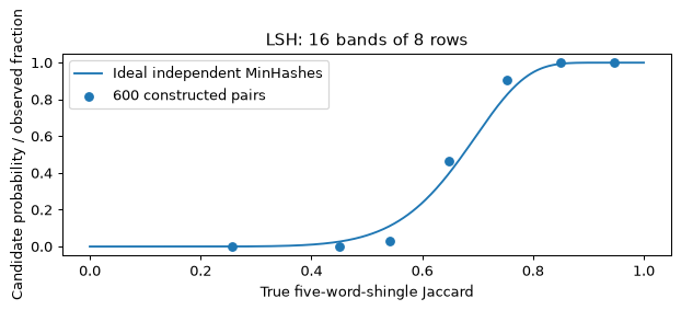
The printed theory column averages the formula at each pair’s actual similarity, rather than substituting a wide bin’s midpoint. All pairs share the same hash family and may share a source story, so the bin counts are not independent Bernoulli trials. The scatter is a diagnostic, not a coverage-validated uncertainty interval.
Verify candidates, cluster and log removals
LSH only proposes candidates. Verify their actual shingle overlap before joining clusters. Union-find keeps the lowest document index in each cluster. Transitive closure can join A to C through B even when A and C fall below the threshold; that is a cluster policy, not a claim that every pair in the cluster passes the cutoff.
For the final pipeline, first remove failed-quality documents, then exact copies among the surviving documents, then verified near-duplicate clusters. Recompute the exact keepers at this stage: an earlier first occurrence may have failed quality.
def cluster_remove(active, threshold):
    active = set(active)
    parent = {i:i for i in active}
    def find(i):
        while parent[i] != i:
            parent[i] = parent[parent[i]]
            i = parent[i]
        return i
    for x,y in sorted(candidates):
        if x in active and y in active and jaccard(sets[x],sets[y]) >= threshold:
            rx,ry = find(x),find(y)
            parent[max(rx,ry)] = min(rx,ry)
    return {i for i in active if find(i) != i}

threshold_results = {}
for threshold in [.7,.8,.9]:
    removed = cluster_remove(range(len(docs)), threshold)
    expected = {copy_id for (source,copy_id),similarity in zip(near_pairs,true_j)
                if similarity >= threshold} | set(range(5600,5800))
    precision = len(removed & expected)/len(removed) if removed else 0
    recall = len(removed & expected)/len(expected) if expected else 0
    threshold_results[str(threshold)] = dict(removed=len(removed),
                                            precision=precision, recall=recall)
    print(f"Threshold {threshold:.1f}: removed {len(removed)}; "
          f"constructed-label precision {precision:.3f}; recall {recall:.3f}")

log = {i:"quality: "+reason for i,reason in enumerate(reasons) if reason}
survivors = [i for i in range(len(docs)) if i not in log]
seen = {}
for i in survivors:
    normal = normalise(docs[i])
    key = (hashlib.sha1(normal.encode()).digest(),normal)
    if key in seen:
        log[i] = "exact copy of document " + str(seen[key])
    else:
        seen[key] = i
before_near = [i for i in survivors if i not in log]
near_removed = cluster_remove(before_near,.8)
for i in near_removed:
    log[i] = "near-duplicate cluster at Jaccard threshold 0.8"
counts = Counter(reason.split(":")[0].split(" of ")[0].split(" at ")[0]
                 for reason in log.values())
print("Pipeline:", len(docs), "in;", dict(counts),
      "removed;", len(docs)-len(log), "out")
for i in sorted(log)[:5]:
    print("document", i, "label", labels[i], "reason", log[i])
metrics = dict(input_docs=len(docs), label_counts=dict(Counter(labels)),
               quality_rejections=sum(r is not None for r in reasons),
               original_rejections=sum(r is not None for r in reasons[:5000]),
               mojibake_flags=len(flagged), repair_successes=repaired,
               exact_duplicates_all_input=len(exact_removed),
               minhash_mae=float(error.mean()), minhash_max_error=float(error.max()),
               candidate_pairs=len(candidates), detection_bins=observations,
               thresholds=threshold_results, pipeline_removed=dict(counts),
               output_docs=len(docs)-len(log))
Path("lab1-metrics.json").write_text(json.dumps(metrics,indent=2),encoding="utf8")
Threshold 0.7: removed 461; constructed-label precision 0.892; recall 0.981
Threshold 0.8: removed 379; constructed-label precision 0.881; recall 1.000
Threshold 0.9: removed 306; constructed-label precision 0.876; recall 1.000
Pipeline: 6400 in; {'quality': 604, 'exact copy': 218, 'near-duplicate cluster': 116} removed; 5462 out
document 65 label clean reason quality: word count
document 200 label clean reason quality: ellipsis lines
document 2838 label clean reason quality: word count
document 5000 label navigation reason quality: alphabetic words
document 5001 label navigation reason quality: alphabetic words
Constructed-label precision compares removals with inserted copies passing the chosen similarity threshold. It is not human-labelled duplicate precision: an original story or junk page can also duplicate another input. Review such apparent false positives instead of assuming that every discrepancy is an algorithm error.
What you should see
The junk classes fail different rules, while some original stories also fail. That is evidence that the heuristic needs a false-positive audit. Encoding artefacts can survive ordinary lexical filters. Exact-copy count can exceed the number of inserted exact copies because some near-copy draws make no effective change.
Candidate rates rise sharply with true shingle similarity. One changed word can alter as many as five shingles, so a modest word-edit rate can produce low Jaccard and escape an aggressive eight-row banding scheme. Candidate generation saves pairwise comparisons at the cost of missed pairs. Verification prevents low-overlap hash coincidences from being treated as duplicates but cannot recover pairs that LSH never proposed.
Try this
- Use 32 bands of four rows and eight bands of sixteen rows, keeping 128 signature values. Compare candidate count and recall, and plot all three theoretical curves.
- Hold out fifty source stories as a mock benchmark. Insert ten edited versions and compare five-word MinHash with a thirteen-word overlap detector. Split duplicate families together before using a corpus for validation.
- Apply the quality rules to a structured technical argument with numbered goals and terse records. Inspect rejected examples before transferring any threshold from web prose to the engineering domain.
Lab 2 — Pretrain a small GPT on TinyStories
Goal. Train a tokenizer and decoder, pack documents, monitor training and validation, score a small cloze test, and prove that a checkpoint restores the optimiser and random sampler as well as the weights. Save a tokenizer, model configuration and measured run record.
This lab repeats the pinned 10 MB TinyStories download from Lab 1 and makes its
own split and tokenizer. Every lab can run in a fresh process. The synthetic
children’s stories are a small training experiment, not evidence about technical
reasoning. Start with QUICK = True (150 steps); set it to False for 600 steps.
Both paths use the same architecture. A free Colab GPU is another option; the code
uses bf16 autocast only when the CUDA device supports it.
Fix the split, tokenizer and packed stream
Hold out 1,000 stories before fitting BPE. Start from all 256 bytes, retain the end-of-text special token, and train a vocabulary of 4,096 on the remaining 20,990 stories. Keep that mapping unchanged for training, scoring and generation. The released validation parquet is this lab’s raw corpus; our split is separate from TinyStories’ original training/validation division.
QUICK = True
import math
import time
import json
from pathlib import Path
from contextlib import nullcontext
import numpy as np
import pandas as pd
import torch
from torch import nn
from torch.nn import functional as F
import matplotlib.pyplot as plt
from tokenizers import Tokenizer, models, trainers, pre_tokenizers, decoders
from huggingface_hub import hf_hub_download

torch.set_num_threads(4)
torch.manual_seed(0)
np.random.seed(0)
device = torch.device("cuda" if torch.cuda.is_available() else "cpu")
use_bf16 = device.type == "cuda" and torch.cuda.is_bf16_supported()

def precision():
    return (torch.autocast("cuda", dtype=torch.bfloat16) if use_bf16
            else nullcontext())

revision = "f54c09fd23315a6f9c86f9dc80f725de7d8f9c64"
path = hf_hub_download(
    "roneneldan/TinyStories",
    "data/validation-00000-of-00001-869c898b519ad725.parquet",
    repo_type="dataset", revision=revision,
)
stories = pd.read_parquet(path)["text"].tolist()
order = np.random.default_rng(0).permutation(len(stories))
train_texts = [stories[i] for i in order[1000:]]
valid_texts = [stories[i] for i in order[:1000]]

def train_tokenizer(texts):
    tokenizer = Tokenizer(models.BPE())
    tokenizer.pre_tokenizer = pre_tokenizers.ByteLevel(add_prefix_space=False)
    tokenizer.decoder = decoders.ByteLevel()
    trainer = trainers.BpeTrainer(
        vocab_size=4096, special_tokens=["<|endoftext|>"],
        initial_alphabet=pre_tokenizers.ByteLevel.alphabet(), show_progress=False,
    )
    tokenizer.train_from_iterator(texts, trainer=trainer)
    return tokenizer

tokenizer = train_tokenizer(train_texts)
eos = tokenizer.token_to_id("<|endoftext|>")

def pack(texts, tok=tokenizer):
    ends = tok.token_to_id("<|endoftext|>")
    encoded = tok.encode_batch(texts)
    lengths = [len(item.ids)+1 for item in encoded]
    stream = np.fromiter(
        (token for item in encoded for token in [*item.ids, ends]),
        dtype=np.uint16, count=sum(lengths),
    )
    return torch.from_numpy(stream.astype(np.int64)), lengths

train_data, lengths = pack(train_texts)
valid_data, _ = pack(valid_texts)
print("Device:", device, "bf16 autocast:", use_bf16)
print("Stories:", len(train_texts), "train;", len(valid_texts), "validation")
print("Vocabulary:", tokenizer.get_vocab_size(), "EOS:", eos)
print("Tokens:", len(train_data), "train;", len(valid_data), "validation")
Device: cpu bf16 autocast: False
Stories: 20990 train; 1000 validation
Vocabulary: 4096 EOS: 0
Tokens: 4650186 train; 228958 validation
Packing appends EOS to each story and concatenates them. Windows can cross an EOS boundary; this experiment permits attention to preceding documents instead of implementing block-diagonal document masking. Every position still has a causal target. Padding whole stories to multiples of 512 would waste the fraction printed below, assuming that stories longer than 512 are split into chunks.
example = "Once upon a time, there was a little girl named Lily."
print("Example tokens:", tokenizer.encode(example).tokens)
characters = sum(map(len,train_texts))
words = sum(len(text.split()) for text in train_texts)
content_tokens = len(train_data)-len(train_texts)
padded = sum(512*math.ceil(length/512) for length in lengths)
print(f"Compression: {characters/content_tokens:.3f} characters/token; "
      f"{content_tokens/words:.3f} tokens/word")
print(f"Padding waste avoided: {1-len(train_data)/padded:.1%}")

# A measured large-matmul baseline, not the hardware's advertised peak.
dtype = torch.bfloat16 if use_bf16 else torch.float32
a = torch.randn(1024,1024,device=device,dtype=dtype)
b = torch.randn_like(a)
for _ in range(3):
    product = a@b
if device.type == "cuda":
    torch.cuda.synchronize()
start = time.perf_counter()
for _ in range(20):
    product = a@b
if device.type == "cuda":
    torch.cuda.synchronize()
matmul_rate = 20*2*1024**3/(time.perf_counter()-start)
print(f"Measured matmul baseline: {matmul_rate/1e9:.1f} GFLOP/s")
Example tokens: ['Once', 'Ġupon', 'Ġa', 'Ġtime', ',', 'Ġthere', 'Ġwas', 'Ġa', 'Ġlittle', 'Ġgirl', 'Ġnamed', 'ĠLily', '.']
Compression: 3.952 characters/token; 1.294 tokens/word
Padding waste avoided: 58.0%
Measured matmul baseline: 509.1 GFLOP/s
On a CPU, model FLOP/s divided by this measured baseline is a utilisation proxy. It is not production MFU, whose denominator is the device’s published peak at the training precision. Matmul size, kernel choice and other running programs affect this measurement; keep it beside the throughput figure rather than treating it as a machine specification.
Declare the decoder and optimiser
This is Module 06’s causal decoder, repeated here for independence: RMSNorm, RoPE, SwiGLU, no biases and tied input/output embeddings. Residual projections start with a smaller standard deviation. The optional QK norms are disabled in this lab; Lab 3 tests them. There is no dropout, making the resume experiment easier to interpret.
class RMSNorm(nn.Module):
    def __init__(self, width):
        super().__init__()
        self.weight = nn.Parameter(torch.ones(width))

    def forward(self, x):
        return F.rms_norm(x, (x.shape[-1],), self.weight, eps=1e-5)

class Attention(nn.Module):
    def __init__(self, d, heads, context, qk_norm=False):
        super().__init__()
        self.heads, self.dh = heads, d//heads
        self.qkv = nn.Linear(d, 3*d, bias=False)
        self.out = nn.Linear(d, d, bias=False)
        self.qnorm = RMSNorm(self.dh) if qk_norm else nn.Identity()
        self.knorm = RMSNorm(self.dh) if qk_norm else nn.Identity()
        angles = torch.outer(torch.arange(context),
                             10000**(-torch.arange(0, self.dh, 2)/self.dh))
        self.register_buffer("cos", angles.cos(), persistent=False)
        self.register_buffer("sin", angles.sin(), persistent=False)
        self.probe = False
        self.max_logit = 0.0

    def rotate(self, x):
        pairs = x.reshape(*x.shape[:-1], self.dh//2, 2)
        a, b = pairs.unbind(-1)
        cos = self.cos[:x.shape[-2]].to(x.dtype)
        sin = self.sin[:x.shape[-2]].to(x.dtype)
        return torch.stack((a*cos-b*sin, a*sin+b*cos), -1).flatten(-2)

    def forward(self, x):
        B,T,d = x.shape
        q,k,v = self.qkv(x).chunk(3, -1)
        q,k,v = [y.view(B,T,self.heads,self.dh).transpose(1,2)
                 for y in (q,k,v)]
        q,k = self.rotate(self.qnorm(q)), self.rotate(self.knorm(k))
        if self.probe:
            with torch.no_grad():
                scores = q.float() @ k.float().transpose(-2,-1)/math.sqrt(self.dh)
                causal = torch.ones(T,T,device=x.device,dtype=torch.bool).tril()
                self.max_logit = scores.masked_select(causal).abs().max().item()
        y = F.scaled_dot_product_attention(q,k,v,is_causal=True)
        return self.out(y.transpose(1,2).contiguous().view(B,T,d))

class Block(nn.Module):
    def __init__(self, d, heads, ff, context, qk_norm=False):
        super().__init__()
        self.n1, self.n2 = RMSNorm(d), RMSNorm(d)
        self.attn = Attention(d,heads,context,qk_norm)
        self.gate = nn.Linear(d,ff,bias=False)
        self.up = nn.Linear(d,ff,bias=False)
        self.down = nn.Linear(ff,d,bias=False)

    def forward(self, x):
        x = x + self.attn(self.n1(x))
        y = self.n2(x)
        return x + self.down(F.silu(self.gate(y))*self.up(y))

class GPT(nn.Module):
    def __init__(self, V=4096, d=256, layers=6, heads=8, ff=688,
                 context=256, qk_norm=False):
        super().__init__()
        assert d%heads == 0 and (d//heads)%2 == 0
        self.context = context
        self.embedding = nn.Embedding(V,d)
        self.blocks = nn.ModuleList(
            [Block(d,heads,ff,context,qk_norm) for _ in range(layers)])
        self.norm = RMSNorm(d)
        self.head = nn.Linear(d,V,bias=False)
        self.head.weight = self.embedding.weight
        for param in self.parameters():
            if param.ndim >= 2:
                nn.init.normal_(param,std=.02)
        for block in self.blocks:
            nn.init.normal_(block.attn.out.weight,std=.02/math.sqrt(2*layers))
            nn.init.normal_(block.down.weight,std=.02/math.sqrt(2*layers))

    def forward(self, tokens):
        x = self.embedding(tokens)
        for block in self.blocks:
            x = block(x)
        return self.head(self.norm(x))

def make_optimizer(model, lr):
    matrices = [p for p in model.parameters() if p.ndim >= 2]
    norms = [p for p in model.parameters() if p.ndim < 2]
    return torch.optim.AdamW(
        [{"params": matrices, "weight_decay": .1},
         {"params": norms, "weight_decay": 0.0}],
        lr=lr, betas=(.9,.95), eps=1e-8,
    )

def batch(stream, generator, T, B=16):
    starts = torch.randint(len(stream)-T, (B,), generator=generator)
    indices = starts[:,None] + torch.arange(T+1)
    windows = stream[indices].to(device)
    return windows[:,:-1], windows[:,1:]

@torch.no_grad()
def evaluate(model, batches):
    was_training = model.training
    model.eval()
    losses = []
    for x,y in batches:
        with precision():
            logits = model(x)
            loss = F.cross_entropy(logits.float().flatten(0,1), y.flatten())
        losses.append(loss.item())
    model.train(was_training)
    return float(np.mean(losses))

def learning_rate(step, steps, warmup, peak):
    if step < warmup:
        return peak*(step+1)/warmup
    fraction = (step-warmup)/max(1,steps-1-warmup)
    return peak*(.1 + .9*(1+math.cos(math.pi*fraction))/2)

@torch.no_grad()
def generate(model, prompt, count=60, temperature=.8, seed=0):
    was_training = model.training
    model.eval()
    ids = tokenizer.encode(prompt).ids
    generator = torch.Generator().manual_seed(seed)
    for _ in range(count):
        tokens = torch.tensor([ids[-model.context:]],device=device)
        with precision():
            logits = model(tokens)[0,-1].float().cpu()
        next_id = torch.multinomial((logits/temperature).softmax(-1),
                                    1,generator=generator).item()
        if next_id == eos:
            break
        ids.append(next_id)
    model.train(was_training)
    return tokenizer.decode(ids)
config = dict(V=4096,d=256,layers=6,heads=8,ff=688,context=256)
torch.manual_seed(0)
model = GPT(**config).to(device)
N = sum(p.numel() for p in model.parameters())
assert N == 5795072
optimizer = make_optimizer(model,3e-3)
print("Parameters:", N)
print("Decayed matrices:",sum(p.numel() for p in optimizer.param_groups[0]["params"]))
print("Undecayed norms:",sum(p.numel() for p in optimizer.param_groups[1]["params"]))
steps, warmup = (150,30) if QUICK else (600,60)
T = config["context"]
train_generator = torch.Generator().manual_seed(0)
valid_generator = torch.Generator().manual_seed(123)
valid_batches = [batch(valid_data,valid_generator,T) for _ in range(20)]
flops_per_token = 6*N + 6*config["layers"]*T*config["d"]
print("Steps:", steps, "tokens/step:",16*T,
      "training FLOPs/token:",flops_per_token)
Parameters: 5795072
Decayed matrices: 5791744
Undecayed norms: 3328
Steps: 150 tokens/step: 4096 training FLOPs/token: 37129728
Score twenty-four explicit cloze items
Each pair below gives the intended answer first. Score each entire continuation by summed conditional log-probability, including its leading space; do not sample an answer or compare only the first token. Assert that appending the option does not change the context tokens. This is a hand-written diagnostic of story vocabulary and simple context use, not an independent benchmark. Most answers are plausible from the last few words alone.
cloze = [
    ('Once upon a time, there was a little girl named', 'Lily', 'table'),
    ('She was very happy because she got a new', 'toy', 'sad'),
    ('The dog wagged its', 'tail', 'book'),
    ('Tom was hungry, so he ate an', 'apple', 'car'),
    ('It was raining, so they took an', 'umbrella', 'elephant'),
    ('At night, the sky was full of', 'stars', 'soup'),
    ('Lily asked, "Can I go to the park?" Mom said, "Yes, you', 'can', 'blue'),
    ('The bird flew up into the', 'sky', 'spoon'),
    ('Ben fell down and hurt his', 'knee', 'cloud'),
    ('They played in the sand at the', 'beach', 'book'),
    ('The ice cream was cold and', 'sweet', 'angry'),
    ('The little boat floated on the', 'water', 'bread'),
    ('He was sad because he lost his', 'ball', 'happy'),
    ('The baby was tired, so she went to', 'sleep', 'fly'),
    ('The fish swam in the', 'pond', 'tree'),
    ('Max wanted to play, but it was time for', 'bed', 'sky'),
    ('The car went fast down the', 'road', 'cake'),
    ('At the end of the day, the sun went', 'down', 'fork'),
    ('Kate lost her red hat in the park. The next day, she went back '
     'to the park to look for her', 'hat', 'dog'),
    ('Ben had a dog and a cat. The dog liked to bark, '
     'and the cat liked to', 'meow', 'bark'),
    ('It was a cold winter day. Outside, the ground was covered with', 'snow', 'sand'),
    ('Lily was sad because her doll was broken. Then Dad fixed it, and '
     'Lily felt', 'happy', 'sad'),
    ('Sam loved to swim. Every day after school, he went to the', 'pool', 'library'),
    ('The sky was dark and full of clouds. Soon it began to', 'rain', 'shine'),
]

@torch.no_grad()
def continuation_score(model, context, option):
    prefix = tokenizer.encode(context).ids
    full = tokenizer.encode(context+" "+option).ids
    assert full[:len(prefix)] == prefix
    ids = torch.tensor([full],device=device)
    with precision():
        logp = model(ids[:,:-1]).float().log_softmax(-1)
    targets = ids[:,1:]
    scores = logp.gather(-1,targets[:,:,None]).squeeze(-1)
    return scores[0,len(prefix)-1:].sum().item()

def cloze_score(model):
    was_training = model.training
    model.eval()
    correct = [continuation_score(model,c,a)>continuation_score(model,c,b)
               for c,a,b in cloze]
    model.train(was_training)
    return sum(correct), sum(correct[:18]), sum(correct[18:])

initial_loss = evaluate(model,valid_batches)
initial_cloze = cloze_score(model)
print(f"Initial validation: {initial_loss:.4f}; uniform ln(V): {math.log(4096):.4f}")
print("Initial cloze (all / local / earlier-context):",initial_cloze)
Initial validation: 8.3274; uniform ln(V): 8.3178
Initial cloze (all / local / earlier-context): (11, 11, 0)
Train, evaluate and checkpoint
Draw random windows with a dedicated CPU generator. They can overlap; validation comes from held-out stories, so low training loss alone is not the test. Log the pre-clipping norm and the learning rate actually used. Fixed validation batches and cloze scoring leave the training sampler untouched.
The checkpoint records the next step to execute, weights, Adam moments, sampler and global random states. Saving only a model is sufficient for inference, but does not recreate the next training update.
def training_step(model, optimizer, generator, step):
    lr = learning_rate(step,steps,warmup,3e-3)
    for group in optimizer.param_groups:
        group["lr"] = lr
    x,y = batch(train_data,generator,T)
    optimizer.zero_grad(set_to_none=True)
    with precision():
        logits = model(x)
        loss = F.cross_entropy(logits.float().flatten(0,1),y.flatten())
    loss.backward()
    norm = nn.utils.clip_grad_norm_(model.parameters(),1.0).item()
    optimizer.step()
    return loss.item(),norm,lr

history, validation, resume_reference = [], [], []
wall_start = time.perf_counter()
interval_seconds = 0.0
midpoint = steps//2
for step in range(steps):
    start = time.perf_counter()
    loss,norm,lr = training_step(model,optimizer,train_generator,step)
    if device.type == "cuda":
        torch.cuda.synchronize()
    interval_seconds += time.perf_counter()-start
    history.append(dict(step=step+1,tokens=(step+1)*16*T,
                        loss=loss,grad_norm=norm,lr=lr))
    if midpoint <= step < midpoint+3:
        resume_reference.append(loss)
    if (step+1)%25 == 0:
        rate = 25*16*T/interval_seconds
        proxy = flops_per_token*rate/matmul_rate
        print(f"Step {step+1:3}; tokens {(step+1)*16*T:7}; loss {loss:.4f}; "
              f"norm {norm:.3f}; lr {lr:.2e}; {rate:.0f} tok/s; proxy {proxy:.1%}")
        interval_seconds = 0.0
    if (step+1)%150 == 0:
        val = evaluate(model,valid_batches)
        cloze_result = cloze_score(model)
        validation.append(dict(step=step+1,tokens=(step+1)*16*T,
                               loss=val,cloze=list(cloze_result)))
        print(f"Validation {step+1}: {val:.4f}; cloze {cloze_result}")
    if step+1 == midpoint:
        torch.save(dict(
            config=config,model=model.state_dict(),optimizer=optimizer.state_dict(),
            next_step=step+1,sampler=train_generator.get_state(),
            torch_rng=torch.get_rng_state(),numpy_rng=np.random.get_state(),
            cuda_rng=torch.cuda.get_rng_state_all() if device.type=="cuda" else [],
        ),"midpoint.pt")

elapsed = time.perf_counter()-wall_start
final_loss = evaluate(model,valid_batches)
print(f"Time: {elapsed:.1f}s; final validation {final_loss:.4f}; "
      f"perplexity {math.exp(final_loss):.2f}")
print("Sample:",generate(model,"Once upon a time",count=120))
Step  25; tokens  102400; loss 5.8707; norm 3.043; lr 2.50e-03; 8102 tok/s; proxy 59.1%
Step  50; tokens  204800; loss 5.2623; norm 1.451; lr 2.83e-03; 8153 tok/s; proxy 59.5%
Step  75; tokens  307200; loss 4.6081; norm 0.821; lr 2.19e-03; 7953 tok/s; proxy 58.0%
Step 100; tokens  409600; loss 4.2007; norm 0.535; lr 1.31e-03; 6285 tok/s; proxy 45.8%
Step 125; tokens  512000; loss 4.2029; norm 0.567; lr 5.84e-04; 6088 tok/s; proxy 44.4%
Step 150; tokens  614400; loss 3.9935; norm 0.506; lr 3.00e-04; 7358 tok/s; proxy 53.7%
Validation 150: 3.9858; cloze (15, 12, 3)
Time: 88.4s; final validation 3.9858; perplexity 53.83
Sample: Once upon a time!" there was a little girl was a little girl called with a tree. He was looked down and wanted to work.
Verify resumption and save the deliverables
Load only this locally created checkpoint. Restoring its trusted Python objects
requires weights_only=False; never use that option on an untrusted file. The
fresh-optimiser control starts with the same weights and draws the same windows,
but omits Adam’s accumulated moments. Its first loss is identical because it is
measured before the first update; later losses reveal the changed trajectory.
def resumed_losses(restore_optimizer):
    saved = torch.load("midpoint.pt",map_location=device,weights_only=False)
    resumed = GPT(**saved["config"]).to(device)
    resumed.load_state_dict(saved["model"])
    opt = make_optimizer(resumed,3e-3)
    if restore_optimizer:
        opt.load_state_dict(saved["optimizer"])
    generator = torch.Generator()
    generator.set_state(saved["sampler"].cpu())
    torch.set_rng_state(saved["torch_rng"].cpu())
    np.random.set_state(saved["numpy_rng"])
    if device.type == "cuda":
        torch.cuda.set_rng_state_all([state.cpu() for state in saved["cuda_rng"]])
    return [training_step(resumed,opt,generator,i)[0]
            for i in range(saved["next_step"],saved["next_step"]+3)]

restored = resumed_losses(True)
fresh = resumed_losses(False)
print("Original:"," ".join(f"{x:.6f}" for x in resume_reference))
print("Restored:"," ".join(f"{x:.6f}" for x in restored))
print("Fresh Adam:"," ".join(f"{x:.6f}" for x in fresh))
maximum_error = max(abs(a-b) for a,b in zip(restored,resume_reference))
print(f"Resume maximum loss error: {maximum_error:.3e}")
assert maximum_error < 1e-5
assert max(abs(a-b) for a,b in zip(fresh,resume_reference)) > 1e-4

torch.save(dict(config=config,model=model.state_dict()),"final-model.pt")
tokenizer.save("tokenizer.json")
metrics = dict(quick=QUICK,parameters=N,config=config,
               train_tokens=len(train_data),valid_tokens=len(valid_data),
               initial_validation=initial_loss,final_validation=final_loss,
               initial_cloze=list(initial_cloze),final_cloze=list(cloze_score(model)),
               elapsed_seconds=elapsed,matmul_flops_per_second=matmul_rate,
               history=history,validation=validation,
               resume_original=resume_reference,resume_restored=restored,
               resume_fresh_optimizer=fresh)
Path("lab2-metrics.json").write_text(json.dumps(metrics,indent=2),encoding="utf8")
fig,ax = plt.subplots(figsize=(7.2,3.6))
ax.plot([r["tokens"] for r in history],[r["loss"] for r in history],
        color="#0072B2",alpha=.65,label="Training batch")
ax.scatter([r["tokens"] for r in validation],[r["loss"] for r in validation],
           color="#D55E00",label="Held-out stories",zorder=3)
ax.set(xlabel="Training tokens seen",ylabel="Cross-entropy (nats/token)",
       title="TinyStories pretraining: loss and learning-rate schedule")
right = ax.twinx()
right.plot([r["tokens"] for r in history],[r["lr"] for r in history],
           color="#009E73",linestyle="--")
right.set_ylabel("Learning rate",color="#009E73")
ax.legend(loc="upper right")
fig.tight_layout()
plt.show()
Original: 4.722644 4.489676 4.691318
Restored: 4.722644 4.489676 4.691318
Fresh Adam: 4.722644 6.282327 5.666222
Resume maximum loss error: 0.000e+00
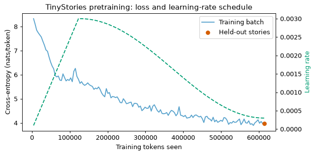
The files live in the directory from which you ran the lab (the lab runner uses
labs/module_08/run_lab2/). Later labs train their own tokenizer and base, so
they do not depend on these files. Preserve the pinned corpus revision and split
alongside the run record if you reuse this checkpoint.
What you should see
In this CPU environment, QUICK held-out loss fell from 8.3274 to 3.9858, with 15/24 cloze answers correct (12/18 local, 3/6 earlier-context). A separate 600-step run reached 2.8327, perplexity 16.99, with 21/24 correct (18/18 and 3/6). That full run also logged validation every 25 steps for the scaling diagnostic; extra evaluations change elapsed time, while leaving the dedicated training sampler untouched. Its three restored losses again matched exactly. Recorded metrics distinguish QUICK from FULL; samples and timing depend on the machine.
Loss starts near the uniform baseline, then falls as the model learns frequent story patterns. The cloze test distinguishes local completion from cases that mention earlier context, but each item changes accuracy by 4.2 percentage points. An improvement on a few questions is not a precise general capability estimate. Samples can resemble stories while making grammatical or factual mistakes.
The complete checkpoint reproduces the next three losses; fresh Adam moments change the second and third. Validation is measured on fixed windows in held-out stories. Those windows are correlated and need not be free of duplicate families across the document split; audit that issue before treating loss differences as precise generalisation estimates.
Try this
- At equal estimated FLOPs, train the 1.33M-parameter shape from Lab 3 on more tokens and compare held-out loss. Include attention in the compute estimate.
- Replace cosine decay with a stable phase and a final linear decay. Record validation just before decay and at the end rather than attributing every improvement to tokens alone.
- On a GPU, enlarge width and batch gradually. Measure memory and throughput, and calculate MFU against the device’s published peak at the precision used.
Lab 3 — Provoke an instability, then diagnose its mechanism
Goal. Raise the learning rate of a small decoder, measure the resulting attention logits and loss, and test warmup, gradient clipping, z-loss and QK normalisation in a controlled sequence. Then compare sensitivity across three learning rates. A fix is useful when it addresses the observed failure mechanism.
This lab downloads the same pinned 10 MB TinyStories file if it is not cached, fits its own tokenizer and repeats the complete decoder declaration. Nine short runs each start from the same seed and see the same windows. Expect several minutes on a laptop CPU; a CUDA device or free Colab session also works.
Repeat the data and model setup
The model is smaller than Lab 2’s: width 128, four layers, four heads, SwiGLU width 352, context 128 and tied embeddings. QK normalisation applies a learned RMSNorm to each query and key before RoPE. A diagnostic switch computes the largest absolute causal attention logit on the final training batch; it does not change the SDPA output or its gradient.
import math
import time
import json
from pathlib import Path
from contextlib import nullcontext
import numpy as np
import pandas as pd
import torch
from torch import nn
from torch.nn import functional as F
import matplotlib.pyplot as plt
from tokenizers import Tokenizer, models, trainers, pre_tokenizers, decoders
from huggingface_hub import hf_hub_download

torch.set_num_threads(4)
torch.manual_seed(0)
np.random.seed(0)
device = torch.device("cuda" if torch.cuda.is_available() else "cpu")
use_bf16 = device.type == "cuda" and torch.cuda.is_bf16_supported()

def precision():
    return (torch.autocast("cuda", dtype=torch.bfloat16) if use_bf16
            else nullcontext())

revision = "f54c09fd23315a6f9c86f9dc80f725de7d8f9c64"
path = hf_hub_download(
    "roneneldan/TinyStories",
    "data/validation-00000-of-00001-869c898b519ad725.parquet",
    repo_type="dataset", revision=revision,
)
stories = pd.read_parquet(path)["text"].tolist()
order = np.random.default_rng(0).permutation(len(stories))
train_texts = [stories[i] for i in order[1000:]]
valid_texts = [stories[i] for i in order[:1000]]

def train_tokenizer(texts):
    tokenizer = Tokenizer(models.BPE())
    tokenizer.pre_tokenizer = pre_tokenizers.ByteLevel(add_prefix_space=False)
    tokenizer.decoder = decoders.ByteLevel()
    trainer = trainers.BpeTrainer(
        vocab_size=4096, special_tokens=["<|endoftext|>"],
        initial_alphabet=pre_tokenizers.ByteLevel.alphabet(), show_progress=False,
    )
    tokenizer.train_from_iterator(texts, trainer=trainer)
    return tokenizer

tokenizer = train_tokenizer(train_texts)
eos = tokenizer.token_to_id("<|endoftext|>")

def pack(texts, tok=tokenizer):
    ends = tok.token_to_id("<|endoftext|>")
    encoded = tok.encode_batch(texts)
    lengths = [len(item.ids)+1 for item in encoded]
    stream = np.fromiter(
        (token for item in encoded for token in [*item.ids, ends]),
        dtype=np.uint16, count=sum(lengths),
    )
    return torch.from_numpy(stream.astype(np.int64)), lengths

train_data, lengths = pack(train_texts)
valid_data, _ = pack(valid_texts)
print("Device:", device, "bf16 autocast:", use_bf16)
print("Stories:", len(train_texts), "train;", len(valid_texts), "validation")
print("Vocabulary:", tokenizer.get_vocab_size(), "EOS:", eos)
print("Tokens:", len(train_data), "train;", len(valid_data), "validation")
Device: cpu bf16 autocast: False
Stories: 20990 train; 1000 validation
Vocabulary: 4096 EOS: 0
Tokens: 4650186 train; 228958 validation
class RMSNorm(nn.Module):
    def __init__(self, width):
        super().__init__()
        self.weight = nn.Parameter(torch.ones(width))

    def forward(self, x):
        return F.rms_norm(x, (x.shape[-1],), self.weight, eps=1e-5)

class Attention(nn.Module):
    def __init__(self, d, heads, context, qk_norm=False):
        super().__init__()
        self.heads, self.dh = heads, d//heads
        self.qkv = nn.Linear(d, 3*d, bias=False)
        self.out = nn.Linear(d, d, bias=False)
        self.qnorm = RMSNorm(self.dh) if qk_norm else nn.Identity()
        self.knorm = RMSNorm(self.dh) if qk_norm else nn.Identity()
        angles = torch.outer(torch.arange(context),
                             10000**(-torch.arange(0, self.dh, 2)/self.dh))
        self.register_buffer("cos", angles.cos(), persistent=False)
        self.register_buffer("sin", angles.sin(), persistent=False)
        self.probe = False
        self.max_logit = 0.0

    def rotate(self, x):
        pairs = x.reshape(*x.shape[:-1], self.dh//2, 2)
        a, b = pairs.unbind(-1)
        cos = self.cos[:x.shape[-2]].to(x.dtype)
        sin = self.sin[:x.shape[-2]].to(x.dtype)
        return torch.stack((a*cos-b*sin, a*sin+b*cos), -1).flatten(-2)

    def forward(self, x):
        B,T,d = x.shape
        q,k,v = self.qkv(x).chunk(3, -1)
        q,k,v = [y.view(B,T,self.heads,self.dh).transpose(1,2)
                 for y in (q,k,v)]
        q,k = self.rotate(self.qnorm(q)), self.rotate(self.knorm(k))
        if self.probe:
            with torch.no_grad():
                scores = q.float() @ k.float().transpose(-2,-1)/math.sqrt(self.dh)
                causal = torch.ones(T,T,device=x.device,dtype=torch.bool).tril()
                self.max_logit = scores.masked_select(causal).abs().max().item()
        y = F.scaled_dot_product_attention(q,k,v,is_causal=True)
        return self.out(y.transpose(1,2).contiguous().view(B,T,d))

class Block(nn.Module):
    def __init__(self, d, heads, ff, context, qk_norm=False):
        super().__init__()
        self.n1, self.n2 = RMSNorm(d), RMSNorm(d)
        self.attn = Attention(d,heads,context,qk_norm)
        self.gate = nn.Linear(d,ff,bias=False)
        self.up = nn.Linear(d,ff,bias=False)
        self.down = nn.Linear(ff,d,bias=False)

    def forward(self, x):
        x = x + self.attn(self.n1(x))
        y = self.n2(x)
        return x + self.down(F.silu(self.gate(y))*self.up(y))

class GPT(nn.Module):
    def __init__(self, V=4096, d=256, layers=6, heads=8, ff=688,
                 context=256, qk_norm=False):
        super().__init__()
        assert d%heads == 0 and (d//heads)%2 == 0
        self.context = context
        self.embedding = nn.Embedding(V,d)
        self.blocks = nn.ModuleList(
            [Block(d,heads,ff,context,qk_norm) for _ in range(layers)])
        self.norm = RMSNorm(d)
        self.head = nn.Linear(d,V,bias=False)
        self.head.weight = self.embedding.weight
        for param in self.parameters():
            if param.ndim >= 2:
                nn.init.normal_(param,std=.02)
        for block in self.blocks:
            nn.init.normal_(block.attn.out.weight,std=.02/math.sqrt(2*layers))
            nn.init.normal_(block.down.weight,std=.02/math.sqrt(2*layers))

    def forward(self, tokens):
        x = self.embedding(tokens)
        for block in self.blocks:
            x = block(x)
        return self.head(self.norm(x))

def make_optimizer(model, lr):
    matrices = [p for p in model.parameters() if p.ndim >= 2]
    norms = [p for p in model.parameters() if p.ndim < 2]
    return torch.optim.AdamW(
        [{"params": matrices, "weight_decay": .1},
         {"params": norms, "weight_decay": 0.0}],
        lr=lr, betas=(.9,.95), eps=1e-8,
    )

def batch(stream, generator, T, B=16):
    starts = torch.randint(len(stream)-T, (B,), generator=generator)
    indices = starts[:,None] + torch.arange(T+1)
    windows = stream[indices].to(device)
    return windows[:,:-1], windows[:,1:]

@torch.no_grad()
def evaluate(model, batches):
    was_training = model.training
    model.eval()
    losses = []
    for x,y in batches:
        with precision():
            logits = model(x)
            loss = F.cross_entropy(logits.float().flatten(0,1), y.flatten())
        losses.append(loss.item())
    model.train(was_training)
    return float(np.mean(losses))

def learning_rate(step, steps, warmup, peak):
    if step < warmup:
        return peak*(step+1)/warmup
    fraction = (step-warmup)/max(1,steps-1-warmup)
    return peak*(.1 + .9*(1+math.cos(math.pi*fraction))/2)

@torch.no_grad()
def generate(model, prompt, count=60, temperature=.8, seed=0):
    was_training = model.training
    model.eval()
    ids = tokenizer.encode(prompt).ids
    generator = torch.Generator().manual_seed(seed)
    for _ in range(count):
        tokens = torch.tensor([ids[-model.context:]],device=device)
        with precision():
            logits = model(tokens)[0,-1].float().cpu()
        next_id = torch.multinomial((logits/temperature).softmax(-1),
                                    1,generator=generator).item()
        if next_id == eos:
            break
        ids.append(next_id)
    model.train(was_training)
    return tokenizer.decode(ids)
Use the first 8,000 stories of the fixed training split to make this experiment smaller. The tokenizer still fits the full training split. The attention probe measures the last batch, not the maximum ever seen over the run.
train_data, _ = pack(train_texts[:8000])
small_config = dict(V=4096,d=128,layers=4,heads=4,ff=352,context=128)
probe_model = GPT(**small_config)
print("Small model parameters:",sum(p.numel() for p in probe_model.parameters()))
print("Training stream:",len(train_data),"tokens")
del probe_model

def run(lr, warmup=0, clip=None, z_loss=0.0, qk_norm=False, steps=150):
    torch.manual_seed(0)
    model = GPT(**small_config,qk_norm=qk_norm).to(device)
    # Decay all parameters in this controlled sweep, including norm gains.
    optimizer = torch.optim.AdamW(model.parameters(),lr=lr,betas=(.9,.95),
                                 eps=1e-8,weight_decay=.1)
    generator = torch.Generator().manual_seed(0)
    losses, norms, normalisers = [], [], []
    start = time.perf_counter()
    for step in range(steps):
        rate = lr*min(1,(step+1)/warmup) if warmup else lr
        for group in optimizer.param_groups:
            group["lr"] = rate
        for layer in model.blocks:
            layer.attn.probe = step == steps-1
        x,y = batch(train_data,generator,128)
        optimizer.zero_grad(set_to_none=True)
        with precision():
            logits = model(x).float()
            ce = F.cross_entropy(logits.flatten(0,1),y.flatten())
            logZ = torch.logsumexp(logits,-1)
            objective = ce + z_loss*logZ.square().mean()
        if not torch.isfinite(objective):
            raise RuntimeError(f"Non-finite objective at lr={lr}, step={step}")
        objective.backward()
        norm = nn.utils.clip_grad_norm_(
            model.parameters(),clip if clip is not None else float("inf"))
        optimizer.step()
        losses.append(ce.item())
        norms.append(norm.item())
        normalisers.append(logZ.detach().mean().item())
    return dict(lr=lr,warmup=warmup,clip=clip,z_loss=z_loss,qk_norm=qk_norm,
                final_loss=float(np.mean(losses[-20:])),worst_loss=max(losses[20:]),
                attention_logit=max(b.attn.max_logit for b in model.blocks),
                logZ=float(np.mean(normalisers[-20:])),max_grad_norm=max(norms),
                seconds=time.perf_counter()-start,losses=losses)
Small model parameters: 1328256
Training stream: 1779818 tokens
Apply the stabilisers cumulatively
Keep the high learning rate fixed while adding one intervention at a time. The last comparison adds only QK norms to a run that already has the other three interventions. Log cross-entropy separately from z-loss so that the objective change does not create an artificial improvement in the comparison.
specs = [
    ("reference",dict(lr=.003)),
    ("high rate",dict(lr=.03)),
    ("+ warmup",dict(lr=.03,warmup=50)),
    ("+ clipping",dict(lr=.03,warmup=50,clip=1.0)),
    ("+ z-loss",dict(lr=.03,warmup=50,clip=1.0,z_loss=1e-4)),
    ("+ QK norm",dict(lr=.03,warmup=50,clip=1.0,z_loss=1e-4,qk_norm=True)),
]
results = {}
print("Condition       final CE   worst CE   |attn logit|  mean logZ  max grad")
for name,settings in specs:
    result = run(**settings)
    results[name] = result
    print(f"{name:15} {result['final_loss']:8.3f} {result['worst_loss']:10.3f} "
          f"{result['attention_logit']:14.1f} {result['logZ']:10.2f} "
          f"{result['max_grad_norm']:9.2f}")

fig,ax = plt.subplots(figsize=(7.2,3.6))
for name,color in [("reference","#0072B2"),("high rate","#D55E00"),
                   ("+ z-loss","#CC79A7"),("+ QK norm","#009E73")]:
    ax.plot(np.arange(1,151),results[name]["losses"],label=name,color=color,alpha=.8)
ax.set(xlabel="Training step",ylabel="Cross-entropy (nats/token)",
       title="High learning rate: distinguish the failure and its intervention")
ax.legend()
fig.tight_layout()
plt.show()
Condition       final CE   worst CE   |attn logit|  mean logZ  max grad
reference          4.273      5.948           28.4       8.92      3.00
high rate          5.234      6.285          971.7       8.22      5.94
+ warmup           5.389      6.313          975.6       8.12      5.97
+ clipping         5.549      6.337          752.7       7.81     16.05
+ z-loss           5.478      6.343         1138.2       7.82     15.77
+ QK norm          4.786      6.151           12.4       8.59      8.76
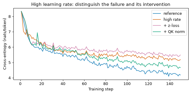
Measure learning-rate sensitivity
Reuse the two already measured bare runs and the high-rate stabilised run. Three new runs complete the sweep. These are training losses after an equal number of steps, not held-out evaluation of nine selected checkpoints; use them to diagnose optimisation, then validate any chosen recipe separately.
rates = [.003,.03,.1]
bare = [results["reference"],results["high rate"],run(.1)]
all_fixes = [run(.003,warmup=50,clip=1,z_loss=1e-4,qk_norm=True),
             results["+ QK norm"],
             run(.1,warmup=50,clip=1,z_loss=1e-4,qk_norm=True)]
print("lr       bare CE   all-fixes CE   bare logit   all-fixes logit")
for lr,a,b in zip(rates,bare,all_fixes):
    print(f"{lr:5.3f} {a['final_loss']:10.3f} {b['final_loss']:14.3f} "
          f"{a['attention_logit']:12.1f} {b['attention_logit']:17.1f}")
metrics = dict(config=small_config,conditions=results,
               sweep_bare=bare,sweep_all=all_fixes)
Path("lab3-metrics.json").write_text(json.dumps(metrics,indent=2),encoding="utf8")
fig,ax = plt.subplots(figsize=(7.2,3.6))
ax.semilogx(rates,[r["final_loss"] for r in bare],"o-",color="#D55E00",
            label="Bare constant rate")
ax.semilogx(rates,[r["final_loss"] for r in all_fixes],"s-",color="#0072B2",
            label="Warmup + clip + z-loss + QK norm")
ax.set(xlabel="Peak learning rate",ylabel="Mean last-20-step loss (nats/token)",
       title="Learning-rate sensitivity of the small TinyStories model")
ax.legend()
fig.tight_layout()
plt.show()
lr       bare CE   all-fixes CE   bare logit   all-fixes logit
0.003      4.273          4.024         28.4               7.0
0.030      5.234          4.786        971.7              12.4
0.100      5.498          4.916       2632.1               8.7
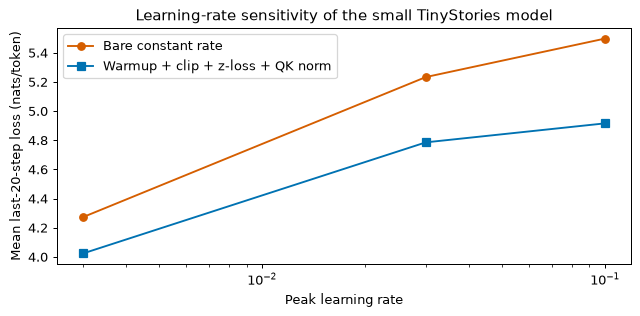
What you should see
Compare loss and attention-logit growth together. Large attention logits can produce sharply concentrated softmax rows and poor optimisation while every logged loss remains finite. Clipping bounds the gradient norm, not the attention logits. Z-loss constrains the output normaliser, not the query/key norms. Warmup changes early update sizes, but does not by itself bound their eventual growth.
QK norms directly control query/key scale; learned gains mean the bound is not the fixed \sqrt{d_h} of unit RMS vectors. Their benefit in this sweep should be read from the measured table, rather than assumed for every architecture and learning rate. An intervention can widen the usable range while leaving a lower learning rate substantially better. Repeating this experiment with different seeds would test how much of each gap is stable.
Try this
- Log attention entropy per head during training. Compare its decline with loss and logit growth; a last-step maximum alone misses the timing of the collapse.
- Remove weight decay and extend training. Compare mean output log-normaliser with and without z-loss while holding QK norms fixed.
- Repeat at width 256 and compare the best rate. Hyperparameter transfer should be tested across model widths, rather than inferred from one successful run.
Lab 4 — A budget and memory calculator
Goal. Turn model shapes into a training budget and memory estimate. Compare ZeRO stages, activation checkpointing, micro-batch sizes, pipeline bubbles and checkpoint intervals. No datasets, model downloads or GPU are required. The formulas are estimates whose assumptions remain visible; a configuration that passes still needs a measured run.
Step 1: parameter counts
Use a bias-free, RMSNorm, SwiGLU decoder. The hypothetical case-study configuration is the same one introduced in Module 07. The other rows let the count be checked at a published shape and at the two planned small training shapes.
import math
import numpy as np

np.random.seed(0)


def params(L, d, n_h, n_kv, d_ff, V, tied=False):
    assert d % n_h == 0 and n_h % n_kv == 0
    attention = 2 * d * d + 2 * d * n_kv * (d // n_h)
    ffn = 3 * d * d_ff
    norms = 2 * d
    blocks = L * (attention + ffn + norms)
    embeddings = V * d * (1 if tied else 2)
    total = blocks + embeddings + d
    return dict(total=total, blocks=blocks, attention=L * attention, ffn=L * ffn,
                norms=L * norms + d, embeddings=embeddings,
                lookup=0 if tied else V * d)


case = dict(L=36, d=4096, n_h=32, n_kv=8, d_ff=15360, V=152064)
llama3 = dict(L=32, d=4096, n_h=32, n_kv=8, d_ff=14336, V=128256)
recipe = dict(L=12, d=768, n_h=12, n_kv=12, d_ff=2048, V=32000, tied=True)
laptop = dict(L=6, d=256, n_h=8, n_kv=8, d_ff=688, V=4096, tied=True)
for name, cfg in (("case study", case), ("Llama-3 shape", llama3),
                  ("small recipe", recipe), ("laptop shape", laptop)):
    c = params(**cfg)
    rule = 12 * cfg["L"] * cfg["d"] ** 2
    print(f"{name:15s} total {c['total']:>13,}, blocks {c['blocks']:>13,}, "
          f"12Ld^2 {rule:>13,}")
assert params(**case)["total"] == 9_550_729_216
assert params(**llama3)["total"] == 8_030_261_248
assert params(**recipe)["total"] == 109_529_856
assert params(**laptop)["total"] == 5_795_072
case study      total 9,550,729,216, blocks 8,305,016,832, 12Ld^2 7,247,757,312
Llama-3 shape   total 8,030,261,248, blocks 6,979,584,000, 12Ld^2 6,442,450,944
small recipe    total   109,529,856, blocks    84,953,088, 12Ld^2    84,934,656
laptop shape    total     5,795,072, blocks     4,746,240, 12Ld^2     4,718,592
The small recipe’s blocks contain 84,953,088 parameters and its tied embedding 24,576,000. The final norm adds 768, giving 109,529,856 in total. A count excluding the final norm would be 109,529,088. The laptop row is a shape calculation; it does not require another lab’s checkpoint.
Step 2: training compute and elapsed time
Module 06, Section 11 owns the FLOP convention. Here its result is a function: exclude lookup-only input embeddings, add causal-average attention, then multiply by training tokens. The shortcut retains every parameter and omits attention.
def train_flops(cfg, tokens, length=8192):
    c = params(**cfg)
    weight = 6 * (c["total"] - c["lookup"])
    attention = 6 * cfg["L"] * cfg["d"] * length
    return (weight + attention) * tokens, 6 * c["total"] * tokens


def compute_for(cfg, tokens, length):
    c = params(**cfg)
    return (6 * (c["total"] - c["lookup"])
            + 6 * cfg["L"] * cfg["d"] * length) * tokens


def gpu_time(compute, sustained, n_gpus):
    gpu_hours = compute / sustained / 3600
    return gpu_hours, gpu_hours / n_gpus


for tokens, gpus in ((2e12, 80), (2e9, 8)):
    compute, quick = train_flops(case, tokens)
    gpu_hours, hours = gpu_time(compute, 4e14, gpus)
    print(f"{tokens:.0e} tokens, {gpus} GPUs: {compute:.3e} FLOPs, "
          f"{gpu_hours:,.1f} GPU-hours, {hours:.2f} hours ({hours / 24:.2f} days)")
    print(f"  6 N_total D shortcut: {quick:.3e} FLOPs, {quick / compute - 1:.1%}")
for mfu in (0.30, 0.40, 0.50):
    compute = compute_for(case, 2e12, 8192)
    _, hours = gpu_time(compute, 989e12 * mfu, 80)
    print(f"assumed MFU {mfu:.0%}: {hours / 24:.1f} days on 80 GPUs")
small_compute = compute_for(recipe, 2.5e9, 2048)
print(f"small recipe: {small_compute:.3e} FLOPs including attention")
2e+12 tokens, 80 GPUs: 1.216e+23 FLOPs, 84,465.3 GPU-hours, 1055.82 hours (43.99 days)
  6 N_total D shortcut: 1.146e+23 FLOPs, -5.8%
2e+09 tokens, 8 GPUs: 1.216e+20 FLOPs, 84.5 GPU-hours, 10.56 hours (0.44 days)
  6 N_total D shortcut: 1.146e+20 FLOPs, -5.8%
assumed MFU 30%: 59.3 days on 80 GPUs
assumed MFU 40%: 44.5 days on 80 GPUs
assumed MFU 50%: 35.6 days on 80 GPUs
small recipe: 1.926e+18 FLOPs including attention
Peak 989 TFLOP/s and sustained 4\times10^{14} FLOP/s are scenario inputs for this calculation. Model FLOP utilisation uses the same arithmetic convention in numerator and denominator. These elapsed times exclude downtime and assume the sustained rate already reflects the selected implementation’s communication and recomputation overhead.
Step 3: model states under sharding
Assume two-byte weights, two-byte gradients and twelve bytes for fp32 master weights plus two fp32 Adam moments. Plain data parallelism replicates all 16 bytes per parameter. ZeRO-1 shards the twelve-byte optimiser state, ZeRO-2 also shards gradients and ZeRO-3 also shards weights. Actual systems may use different gradient dtypes or master weights.
def model_states(N, replicas, stage):
    assert replicas >= 1
    if stage == "DP":
        return N * 16
    if stage == 1:
        return N * (4 + 12 / replicas)
    if stage == 2:
        return N * (2 + 14 / replicas)
    if stage == 3:
        return N * 16 / replicas
    raise ValueError("stage must be DP, 1, 2 or 3")


N = params(**case)["total"]
for replicas in (8, 64, 80):
    sizes = [model_states(N, replicas, stage) / 1e9 for stage in ("DP", 1, 2, 3)]
    print(f"{replicas:2d} GPUs: DP, ZeRO-1, ZeRO-2, ZeRO-3 GB "
          + ", ".join(f"{size:.1f}" for size in sizes))
 8 GPUs: DP, ZeRO-1, ZeRO-2, ZeRO-3 GB 152.8, 52.5, 35.8, 19.1
64 GPUs: DP, ZeRO-1, ZeRO-2, ZeRO-3 GB 152.8, 40.0, 21.2, 2.4
80 GPUs: DP, ZeRO-1, ZeRO-2, ZeRO-3 GB 152.8, 39.6, 20.8, 1.9
ZeRO-3’s permanent weight shard is not its peak allocation. Computing a layer requires gathering its weights; communication buffers and overlapping gathers need extra memory. The fit table below is a component estimate, not a guarantee from the allocator.
Step 4: activations, logits and fits
The approximate saved-activation budget for this recipe is BTL(12d+4n_{\text{kv}}d_{\text{head}}+6d_{\text{ff}}) bytes with fused attention. Full checkpointing saves bf16 layer inputs and retains one recomputed layer’s workspace. The separate logits estimate reserves four bytes per vocabulary logit for fp32 loss computation. A fused loss can require less; extra materialised probabilities can require more.
def activations(cfg, T, micro_batch, checkpoint=False, flash=True):
    L, d = cfg["L"], cfg["d"]
    kv_width = cfg["n_kv"] * (d // cfg["n_h"])
    layer = micro_batch * T * (12 * d + 4 * kv_width + 6 * cfg["d_ff"])
    if not flash:
        layer += 2 * micro_batch * cfg["n_h"] * T * T
    if checkpoint:
        return 2 * micro_batch * T * d * L + layer
    return L * layer


def logits_bytes(cfg, T, micro_batch):
    return 4 * micro_batch * T * cfg["V"]


print(f"case activations: {activations(case, 8192, 1) / 1e9:.2f} GB")
print(f"case checkpointed: {activations(case, 8192, 1, True) / 1e9:.2f} GB")
print(f"case logits: {logits_bytes(case, 8192, 1) / 1e9:.2f} GB")
probabilities = 2 * case["L"] * case["n_h"] * 8192 ** 2
print(f"additional dense bf16 attention probabilities: {probabilities / 1e9:.1f} GB")


def fit(name, cfg, replicas, stage, T, micro_batch, checkpoint, capacity):
    states = model_states(params(**cfg)["total"], replicas, stage)
    acts = activations(cfg, T, micro_batch, checkpoint)
    logits = logits_bytes(cfg, T, micro_batch)
    total = (states + acts + logits) / 1e9
    print(f"{name:27s} states {states / 1e9:5.2f}, acts {acts / 1e9:5.2f}, "
          f"logits {logits / 1e9:4.2f}, total {total:5.2f} GB; "
          f"under {capacity} GB: {total < capacity}")
    return total


fit("case ZeRO-3, 8 GPUs", case, 8, 3, 8192, 1, False, 80)
fit("case ZeRO-3, checkpointed", case, 8, 3, 8192, 1, True, 80)
fit("case ZeRO-1, 80 GPUs", case, 80, 1, 8192, 1, False, 80)
for micro_batch in (16, 32):
    fit(f"small recipe batch {micro_batch}", recipe, 1, "DP", 2048,
        micro_batch, False, 24)
case activations: 42.88 GB
case checkpointed: 3.61 GB
case logits: 4.98 GB
additional dense bf16 attention probabilities: 154.6 GB
case ZeRO-3, 8 GPUs         states 19.10, acts 42.88, logits 4.98, total 66.97 GB; under 80 GB: True
case ZeRO-3, checkpointed   states 19.10, acts  3.61, logits 4.98, total 27.69 GB; under 80 GB: True
case ZeRO-1, 80 GPUs        states 39.64, acts 42.88, logits 4.98, total 87.50 GB; under 80 GB: False
small recipe batch 16       states  1.75, acts  9.66, logits 4.19, total 15.61 GB; under 24 GB: True
small recipe batch 32       states  1.75, acts 19.33, logits 8.39, total 29.47 GB; under 24 GB: False
The numbers exclude allocator fragmentation, communication buffers, temporary layer gathers and other framework allocations. Leave headroom and measure peak memory. Reducing micro-batch size with gradient accumulation preserves the chosen global token batch while reducing activations; it does not reduce permanent optimiser state.
Step 5: pipeline bubbles and recovery intervals
For an ideal balanced pipeline with p stages and m micro-batches, the simple bubble fraction is (p-1)/(m+p-1). Actual schedules, uneven layers and interleaving change it. For checkpoint write time \delta and mean time between interruptions M, the approximate overhead is \delta/\tau+\tau/(2M). Differentiating with respect to the interval \tau gives \tau^*=\sqrt{2\delta M}.
def bubble(stages, micro_batches):
    return (stages - 1) / (micro_batches + stages - 1)


def young_interval(write_seconds, mtbf_seconds):
    return math.sqrt(2 * write_seconds * mtbf_seconds)


for stages, micro_batches in ((4, 4), (4, 16), (8, 8), (8, 64)):
    print(f"pipeline p={stages}, m={micro_batches}: "
          f"bubble {bubble(stages, micro_batches):.1%}")
for mtbf_hours in (3.09, 633):
    interval = young_interval(60, mtbf_hours * 3600)
    overhead = 60 / interval + interval / (2 * mtbf_hours * 3600)
    print(f"MTBF {mtbf_hours:.2f} hours: checkpoint every {interval / 60:.1f} minutes "
          f"({interval / 3600:.2f} hours), estimated overhead {overhead:.1%}")
pipeline p=4, m=4: bubble 42.9%
pipeline p=4, m=16: bubble 15.8%
pipeline p=8, m=8: bubble 46.7%
pipeline p=8, m=64: bubble 9.9%
MTBF 3.09 hours: checkpoint every 19.3 minutes (0.32 hours), estimated overhead 10.4%
MTBF 633.00 hours: checkpoint every 275.6 minutes (4.59 hours), estimated overhead 0.7%
The interruption rates are assumed scenarios. Independent per-device failure scaling is a rough planning model; shared network and storage failures need not follow it. The interval formula omits restart time and assumes complete, restorable checkpoints. Test recovery of optimiser, scheduler, RNG and data-loader state before a long run.
Step 6: reproduce the five-row shortcut table
Keep this table separate from the architecture-aware estimates above. It uses the rounded 9.5B parameter count and 6ND throughout, matching Section 1’s quick first pass. The rows are planning scenarios, not records of completed training runs.
shortcut_rows = [
    ("9.5B / 190B", 9.5e9, 190e9, 16),
    ("9.5B / 2T", 9.5e9, 2e12, 80),
    ("9.5B / 15T", 9.5e9, 15e12, 80),
    ("1B / 20B", 1e9, 20e9, 4),
    ("9.5B CPT / 2B", 9.5e9, 2e9, 8),
]
print("Shortcut scenario   FLOPs       GPU-hours GPUs     days")
for name, N, D, gpus in shortcut_rows:
    compute = 6*N*D
    gpu_hours, hours = gpu_time(compute, 4e14, gpus)
    print(f"{name:18} {compute:9.3e} {gpu_hours:11,.1f} "
          f"{gpus:4d} {hours/24:8.2f}")
Shortcut scenario   FLOPs       GPU-hours GPUs     days
9.5B / 190B        1.083e+22     7,520.8   16    19.59
9.5B / 2T          1.140e+23    79,166.7   80    41.23
9.5B / 15T         8.550e+23   593,750.0   80   309.24
1B / 20B           1.200e+20        83.3    4     0.87
9.5B CPT / 2B      1.140e+20        79.2    8     0.41
The 2T shortcut gives 41.2 days rather than the series rule’s 44.0 days at the same sustained throughput. Rounding a count and omitting attention are different approximations; retain the labels when copying either result into a budget.
Step 7: training allocation and equal-loss payback
Use Module 07’s published parametric law, with raw parameter and token counts. Its budget variable is C_6=6ND, so it does not use the architecture-aware FLOP function. At fixed C_6, compare the analytic fitted minimum and the point constrained to twenty tokens per parameter. Then solve for the smallest training budget whose fitted optimum reaches the case study’s predicted loss.
This equal-loss optimum can cost less to train but more per served token. Using the same approximate serving charge of 2N, solve C_6+2NS=C'_6+2N'S for the served-token break-even. A fixed-budget minimum has a different loss and is not the right comparison for this equal-quality question.
def chinchilla_loss(N, D):
    return 1.69 + 406.4/N**.34 + 410.7/D**.28

def chinchilla_optimum(C):
    N = (.34*406.4/(.28*410.7))**(1/(.34+.28))*(C/6)**(.28/(.34+.28))
    return N, C/(6*N)

def equal_loss_payback(N, D):
    target = chinchilla_loss(N, D)
    lo, hi = 15.0, 28.0
    assert chinchilla_loss(*chinchilla_optimum(10**lo)) > target
    assert chinchilla_loss(*chinchilla_optimum(10**hi)) < target
    for _ in range(80):
        middle = (lo+hi)/2
        minimum = chinchilla_loss(*chinchilla_optimum(10**middle))
        if minimum > target:
            lo = middle
        else:
            hi = middle
    Cprime = 10**((lo+hi)/2)
    Nprime, Dprime = chinchilla_optimum(Cprime)
    assert abs(chinchilla_loss(Nprime,Dprime)-target) < 1e-10
    if N < Nprime*(1-1e-8):
        status = "positive served-token break-even"
        served = (6*N*D-Cprime)/(2*(Nprime-N))
    elif N > Nprime*(1+1e-8):
        status = "original allocation costs more to train and serve"
        served = None
    else:
        status = "already at the fitted equal-loss optimum"
        served = None
    return dict(N=Nprime,D=Dprime,C=Cprime,served=served,status=status)

N = params(**case)["total"]
D = 2e12
C6 = 6*N*D
Nopt,Dopt = chinchilla_optimum(C6)
N20 = math.sqrt(C6/120)
D20 = 20*N20
for name,n,tokens in [("case study",N,D), ("fixed-budget fitted",Nopt,Dopt),
                      ("fixed-budget 20/token",N20,D20)]:
    print(f"{name:23} N {n/1e9:7.3f}B; D {tokens/1e12:6.3f}T; "
          f"loss {chinchilla_loss(n,tokens):.6f}")
payback = equal_loss_payback(N,D)
print(f"Equal-loss fitted: N {payback['N']/1e9:.3f}B; "
      f"D {payback['D']/1e12:.3f}T; C6 {payback['C']:.3e}")
print("Status:",payback["status"])
if payback["served"] is not None:
    print("Served-token break-even:",f"{payback['served']:.3e}")
case study              N   9.551B; D  2.000T; loss 2.001990
fixed-budget fitted     N  15.526B; D  1.230T; loss 1.998483
fixed-budget 20/token   N  30.904B; D  0.618T; loss 2.005373
Equal-loss fitted: N 15.018B; D 1.182T; C6 1.065e+23
Status: positive served-token break-even
Served-token break-even: 7.439e+11
These are extrapolated predictions: both the size and token counts extend beyond the original fitting experiments. The break-even compares model arithmetic, excluding attention, quantisation, capacity, batching and prices. It does not say that either model achieves the same score on the team’s safety-case evaluation. The analogous planner exposes the same assumptions interactively.
What you should see
The 2T-token base plan costs about 1.22\times10^{23} model FLOPs; the 2B-token continued-pretraining plan costs a thousandth as much. On eight GPUs the case-study state estimates are 152.8, 52.5, 35.8 and 19.1 GB for DP and ZeRO stages 1–3. Saved activations drop from about 42.9 GB to 3.61 GB with full checkpointing. These savings cost recomputation and do not include all runtime allocations.
Try this
- Sweep micro-batch size and plot total memory with and without checkpointing. Keep a separately labelled allowance for measured temporary and communication allocations.
- Change gradients to fp32 and add another fp32 logits-sized loss intermediate to see which apparent fits disappear.
- Add an eight-expert, top-two FFN. Separate total stored weights from active compute; sharding and capacity must account for all experts, including those not selected.
Lab 5 — Continued pretraining with and without replay
Goal. Train a small story-language base inside this lab, adapt it to synthetic safety-case text, and measure domain adaptation and forgetting across replay ratios and learning rates. Compare each run with a gate fixed before training.
Use the same pinned 10 MB TinyStories file, downloaded if absent. This lab trains its own tokenizer and base; it does not read Lab 2’s checkpoint. Expect a few minutes on a CPU or use a free Colab GPU. The generated engineering statements are fictional training strings, including their claimed evidence and integrity targets. They cannot establish that a real system meets a safety requirement.
Repeat the independent base setup
Repeat the model declaration to make the lab runnable by itself. The base uses width 128, four layers, four heads, feed-forward width 352 and context 128. Its tokenizer is fitted on general stories only and stays fixed throughout adaptation.
import math
import time
import json
from pathlib import Path
from contextlib import nullcontext
import numpy as np
import pandas as pd
import torch
from torch import nn
from torch.nn import functional as F
import matplotlib.pyplot as plt
from tokenizers import Tokenizer, models, trainers, pre_tokenizers, decoders
from huggingface_hub import hf_hub_download

torch.set_num_threads(4)
torch.manual_seed(0)
np.random.seed(0)
device = torch.device("cuda" if torch.cuda.is_available() else "cpu")
use_bf16 = device.type == "cuda" and torch.cuda.is_bf16_supported()

def precision():
    return (torch.autocast("cuda", dtype=torch.bfloat16) if use_bf16
            else nullcontext())

revision = "f54c09fd23315a6f9c86f9dc80f725de7d8f9c64"
path = hf_hub_download(
    "roneneldan/TinyStories",
    "data/validation-00000-of-00001-869c898b519ad725.parquet",
    repo_type="dataset", revision=revision,
)
stories = pd.read_parquet(path)["text"].tolist()
order = np.random.default_rng(0).permutation(len(stories))
train_texts = [stories[i] for i in order[1000:]]
valid_texts = [stories[i] for i in order[:1000]]

def train_tokenizer(texts):
    tokenizer = Tokenizer(models.BPE())
    tokenizer.pre_tokenizer = pre_tokenizers.ByteLevel(add_prefix_space=False)
    tokenizer.decoder = decoders.ByteLevel()
    trainer = trainers.BpeTrainer(
        vocab_size=4096, special_tokens=["<|endoftext|>"],
        initial_alphabet=pre_tokenizers.ByteLevel.alphabet(), show_progress=False,
    )
    tokenizer.train_from_iterator(texts, trainer=trainer)
    return tokenizer

tokenizer = train_tokenizer(train_texts)
eos = tokenizer.token_to_id("<|endoftext|>")

def pack(texts, tok=tokenizer):
    ends = tok.token_to_id("<|endoftext|>")
    encoded = tok.encode_batch(texts)
    lengths = [len(item.ids)+1 for item in encoded]
    stream = np.fromiter(
        (token for item in encoded for token in [*item.ids, ends]),
        dtype=np.uint16, count=sum(lengths),
    )
    return torch.from_numpy(stream.astype(np.int64)), lengths

train_data, lengths = pack(train_texts)
valid_data, _ = pack(valid_texts)
print("Device:", device, "bf16 autocast:", use_bf16)
print("Stories:", len(train_texts), "train;", len(valid_texts), "validation")
print("Vocabulary:", tokenizer.get_vocab_size(), "EOS:", eos)
print("Tokens:", len(train_data), "train;", len(valid_data), "validation")
Device: cpu bf16 autocast: False
Stories: 20990 train; 1000 validation
Vocabulary: 4096 EOS: 0
Tokens: 4650186 train; 228958 validation
class RMSNorm(nn.Module):
    def __init__(self, width):
        super().__init__()
        self.weight = nn.Parameter(torch.ones(width))

    def forward(self, x):
        return F.rms_norm(x, (x.shape[-1],), self.weight, eps=1e-5)

class Attention(nn.Module):
    def __init__(self, d, heads, context, qk_norm=False):
        super().__init__()
        self.heads, self.dh = heads, d//heads
        self.qkv = nn.Linear(d, 3*d, bias=False)
        self.out = nn.Linear(d, d, bias=False)
        self.qnorm = RMSNorm(self.dh) if qk_norm else nn.Identity()
        self.knorm = RMSNorm(self.dh) if qk_norm else nn.Identity()
        angles = torch.outer(torch.arange(context),
                             10000**(-torch.arange(0, self.dh, 2)/self.dh))
        self.register_buffer("cos", angles.cos(), persistent=False)
        self.register_buffer("sin", angles.sin(), persistent=False)
        self.probe = False
        self.max_logit = 0.0

    def rotate(self, x):
        pairs = x.reshape(*x.shape[:-1], self.dh//2, 2)
        a, b = pairs.unbind(-1)
        cos = self.cos[:x.shape[-2]].to(x.dtype)
        sin = self.sin[:x.shape[-2]].to(x.dtype)
        return torch.stack((a*cos-b*sin, a*sin+b*cos), -1).flatten(-2)

    def forward(self, x):
        B,T,d = x.shape
        q,k,v = self.qkv(x).chunk(3, -1)
        q,k,v = [y.view(B,T,self.heads,self.dh).transpose(1,2)
                 for y in (q,k,v)]
        q,k = self.rotate(self.qnorm(q)), self.rotate(self.knorm(k))
        if self.probe:
            with torch.no_grad():
                scores = q.float() @ k.float().transpose(-2,-1)/math.sqrt(self.dh)
                causal = torch.ones(T,T,device=x.device,dtype=torch.bool).tril()
                self.max_logit = scores.masked_select(causal).abs().max().item()
        y = F.scaled_dot_product_attention(q,k,v,is_causal=True)
        return self.out(y.transpose(1,2).contiguous().view(B,T,d))

class Block(nn.Module):
    def __init__(self, d, heads, ff, context, qk_norm=False):
        super().__init__()
        self.n1, self.n2 = RMSNorm(d), RMSNorm(d)
        self.attn = Attention(d,heads,context,qk_norm)
        self.gate = nn.Linear(d,ff,bias=False)
        self.up = nn.Linear(d,ff,bias=False)
        self.down = nn.Linear(ff,d,bias=False)

    def forward(self, x):
        x = x + self.attn(self.n1(x))
        y = self.n2(x)
        return x + self.down(F.silu(self.gate(y))*self.up(y))

class GPT(nn.Module):
    def __init__(self, V=4096, d=256, layers=6, heads=8, ff=688,
                 context=256, qk_norm=False):
        super().__init__()
        assert d%heads == 0 and (d//heads)%2 == 0
        self.context = context
        self.embedding = nn.Embedding(V,d)
        self.blocks = nn.ModuleList(
            [Block(d,heads,ff,context,qk_norm) for _ in range(layers)])
        self.norm = RMSNorm(d)
        self.head = nn.Linear(d,V,bias=False)
        self.head.weight = self.embedding.weight
        for param in self.parameters():
            if param.ndim >= 2:
                nn.init.normal_(param,std=.02)
        for block in self.blocks:
            nn.init.normal_(block.attn.out.weight,std=.02/math.sqrt(2*layers))
            nn.init.normal_(block.down.weight,std=.02/math.sqrt(2*layers))

    def forward(self, tokens):
        x = self.embedding(tokens)
        for block in self.blocks:
            x = block(x)
        return self.head(self.norm(x))

def make_optimizer(model, lr):
    matrices = [p for p in model.parameters() if p.ndim >= 2]
    norms = [p for p in model.parameters() if p.ndim < 2]
    return torch.optim.AdamW(
        [{"params": matrices, "weight_decay": .1},
         {"params": norms, "weight_decay": 0.0}],
        lr=lr, betas=(.9,.95), eps=1e-8,
    )

def batch(stream, generator, T, B=16):
    starts = torch.randint(len(stream)-T, (B,), generator=generator)
    indices = starts[:,None] + torch.arange(T+1)
    windows = stream[indices].to(device)
    return windows[:,:-1], windows[:,1:]

@torch.no_grad()
def evaluate(model, batches):
    was_training = model.training
    model.eval()
    losses = []
    for x,y in batches:
        with precision():
            logits = model(x)
            loss = F.cross_entropy(logits.float().flatten(0,1), y.flatten())
        losses.append(loss.item())
    model.train(was_training)
    return float(np.mean(losses))

def learning_rate(step, steps, warmup, peak):
    if step < warmup:
        return peak*(step+1)/warmup
    fraction = (step-warmup)/max(1,steps-1-warmup)
    return peak*(.1 + .9*(1+math.cos(math.pi*fraction))/2)

@torch.no_grad()
def generate(model, prompt, count=60, temperature=.8, seed=0):
    was_training = model.training
    model.eval()
    ids = tokenizer.encode(prompt).ids
    generator = torch.Generator().manual_seed(seed)
    for _ in range(count):
        tokens = torch.tensor([ids[-model.context:]],device=device)
        with precision():
            logits = model(tokens)[0,-1].float().cpu()
        next_id = torch.multinomial((logits/temperature).softmax(-1),
                                    1,generator=generator).item()
        if next_id == eos:
            break
        ids.append(next_id)
    model.train(was_training)
    return tokenizer.decode(ids)
Generate domain text and audit tokenizer fit
Eight toy systems give the corpus varied engineering vocabulary. The first is the case study’s pressure-relief system. Random causes, mitigations, evidence labels and timing claims create combinations of the same templates. Hold out 300 distinct documents, and explicitly exclude exact copies across the split. Shared templates make this an easy adaptation experiment; the held-out loss is not a test of whether the generated arguments are sound.
systems = [
    ("the pressure-relief system","a chemical plant","SIL 3",
     ["overpressure of the reactor vessel","a relief valve that fails to open",
      "a blocked vent line"]),
    ("a braking controller","a road vehicle","ASIL D",
     ["loss of braking","unintended braking","a stuck brake actuator"]),
    ("a reactor protection system","a power station","SIL 3",
     ["failure to shut down","a missed trip signal","a sensor disagreement"]),
    ("a flight control computer","an aircraft","DAL A",
     ["loss of control","an erroneous command","a frozen input"]),
    ("a railway interlocking","a railway station","SIL 3",
     ["a conflicting route","a wrong signal aspect","an unlocked point"]),
    ("a battery management system","a road vehicle","ASIL B",
     ["thermal runaway","overcharging","an isolation fault"]),
    ("a robot arm controller","a factory","SIL 2",
     ["unexpected motion","a trapped operator","an overspeed condition"]),
    ("a ventilator","a hospital","a specified integrity target",
     ["loss of airflow","excess pressure","a missed alarm"]),
]
causes = ["a stuck sensor","a corrupted message","a timing fault",
          "a failed actuator","an incorrect configuration","a software defect",
          "a disconnected cable","a power interruption"]
mitigations = ["a hardware watchdog that forces a safe state",
               "an independent shutdown channel","a checked redundant sensor",
               "a monitored interlock","a periodic diagnostic test",
               "a fail-safe actuator","a range and timing check"]
evidence = ["Fault tree analysis","Failure modes and effects analysis",
            "An integration test","A requirements review",
            "A fault-injection test","An independent assessment"]
rng = np.random.default_rng(0)
documents, seen = [], set()
while len(documents) < 3300:
    index = len(documents)%len(systems)
    system,environment,target,hazards = systems[index]
    hazard = hazards[0] if not documents else str(rng.choice(hazards))
    cause = str(rng.choice(causes))
    mitigation = str(rng.choice(mitigations))
    proof = str(rng.choice(evidence))
    delay = int(rng.choice([10,20,50,100,200,500,1000]))
    document = "\n".join([
        f"Context C1: The system is {system} operating in {environment}.",
        f"Goal G1: {system.capitalize()} is acceptably safe in its environment.",
        f"Context C2: The illustrative integrity target is {target}.",
        f"Strategy S1: Argue over identified hazards and their mitigations.",
        f"Goal G2: The hazard of {hazard} is acceptably mitigated.",
        f"Assumption A1: A single fault such as {cause} can initiate the hazard.",
        f"Strategy S2: Use {mitigation} and independent diagnostic coverage.",
        f"Goal G3: The fault is detected and a safe state reached within {delay} ms.",
        f"Solution Sn1: {proof} shows that {mitigation} detects the fault "
        f"within {delay} ms.",
        "Justification J1: The claimed evidence must be checked against the "
        "requirements, operating assumptions and configuration of the system.",
        "Context C3: This is synthetic tutorial text; the evidence is not real.",
    ])
    if document not in seen:
        documents.append(document)
        seen.add(document)
domain_train,domain_valid = documents[:3000],documents[3000:]
assert not set(domain_train)&set(domain_valid)
domain_data,_ = pack(domain_train)
domain_valid_data,_ = pack(domain_valid)
print(documents[0])
print("Domain tokens:",len(domain_data),"train;",len(domain_valid_data),"validation")

def tokens_per_word(tok,texts):
    encoded = tok.encode_batch(texts)
    return sum(len(x.ids) for x in encoded)/sum(len(x.split()) for x in texts)

mixed_texts = train_texts[:12000]+domain_train
mixed_tokenizer = train_tokenizer(mixed_texts)
fraction = sum(map(len,domain_train))/sum(map(len,mixed_texts))
fit = {}
for name,tok in [("story tokenizer",tokenizer),("mixed tokenizer",mixed_tokenizer)]:
    general = tokens_per_word(tok,valid_texts)
    domain = tokens_per_word(tok,domain_valid)
    fit[name] = dict(general=general,domain=domain)
    print(f"{name:16}: general {general:.3f}; domain {domain:.3f} tokens/word")
print(f"Domain character share of mixed-tokenizer training: {fraction:.1%}")
Context C1: The system is the pressure-relief system operating in a chemical plant.
Goal G1: The pressure-relief system is acceptably safe in its environment.
Context C2: The illustrative integrity target is SIL 3.
Strategy S1: Argue over identified hazards and their mitigations.
Goal G2: The hazard of overpressure of the reactor vessel is acceptably mitigated.
Assumption A1: A single fault such as a disconnected cable can initiate the hazard.
Strategy S2: Use a periodic diagnostic test and independent diagnostic coverage.
Goal G3: The fault is detected and a safe state reached within 20 ms.
Solution Sn1: A requirements review shows that a periodic diagnostic test detects the fault within 20 ms.
Justification J1: The claimed evidence must be checked against the requirements, operating assumptions and configuration of the system.
Context C3: This is synthetic tutorial text; the evidence is not real.
Domain tokens: 1075107 train; 107470 validation
story tokenizer : general 1.296; domain 2.535 tokens/word
mixed tokenizer : general 1.304; domain 1.329 tokens/word
Domain character share of mixed-tokenizer training: 20.4%
The mixed tokenizer is a diagnostic only. Replacing token ids underneath the story base would change what its embedding and output rows mean. Adapting a tokenizer requires an explicit embedding transition and more training; this lab keeps the original vocabulary to isolate replay and learning rate.
Train the small base and freeze the baseline
Train 400 steps on stories with warmup-cosine, matrix-only weight decay and clipping. Evaluate ten fixed batches each of general and domain validation. For this toy exercise, write the gate now: at least a one-nat domain-loss reduction and at most a 0.20-nat general-loss rise. This is a diagnostic gate, not the real case study’s task-level acceptance rule.
config = dict(V=4096,d=128,layers=4,heads=4,ff=352,context=128)
torch.manual_seed(0)
base = GPT(**config).to(device)
print("Base parameters:",sum(p.numel() for p in base.parameters()))
optimizer = make_optimizer(base,3e-3)
generator = torch.Generator().manual_seed(0)
general_generator = torch.Generator().manual_seed(123)
domain_generator = torch.Generator().manual_seed(456)
general_batches = [batch(valid_data,general_generator,128) for _ in range(10)]
domain_batches = [batch(domain_valid_data,domain_generator,128) for _ in range(10)]
start = time.perf_counter()
for step in range(400):
    lr = learning_rate(step,400,30,3e-3)
    for group in optimizer.param_groups:
        group["lr"] = lr
    x,y = batch(train_data,generator,128)
    optimizer.zero_grad(set_to_none=True)
    with precision():
        logits = base(x)
        loss = F.cross_entropy(logits.float().flatten(0,1),y.flatten())
    loss.backward()
    nn.utils.clip_grad_norm_(base.parameters(),1.0)
    optimizer.step()
    if (step+1)%100 == 0:
        print(f"Base step {step+1}: training loss {loss.item():.4f}")
baseline = dict(general=evaluate(base,general_batches),
                domain=evaluate(base,domain_batches))
base_state = {key:value.detach().cpu().clone()
              for key,value in base.state_dict().items()}
print(f"Base time {time.perf_counter()-start:.1f}s; "
      f"general {baseline['general']:.4f}; domain {baseline['domain']:.4f}")
print("Gate fixed: domain reduction >= 1.00 nat; general rise <= 0.20 nat")
Base parameters: 1328256
Base step 100: training loss 4.5289
Base step 200: training loss 4.0240
Base step 300: training loss 3.6192
Base step 400: training loss 3.5745
Base time 31.2s; general 3.5098; domain 7.0185
Gate fixed: domain reduction >= 1.00 nat; general rise <= 0.20 nat
Continue from identical weights, varying replay and peak rate
Each continued run starts with fresh Adam state, 10 warmup steps and 100 total updates. Each sequence comes wholly from general or domain data; replay is a Bernoulli draw per sequence, not a forced exact fraction per batch. The same sampler seed aligns the candidate windows across runs. Re-evaluate the same held-out batches, then apply the already declared gate.
def continue_run(replay,peak):
    torch.manual_seed(0)
    model = GPT(**config).to(device)
    model.load_state_dict(base_state)
    optimizer = make_optimizer(model,peak)
    sampler = torch.Generator().manual_seed(0)
    actual_general = 0
    for step in range(100):
        mask = torch.rand(16,generator=sampler) < replay
        gx,gy = batch(train_data,sampler,128)
        dx,dy = batch(domain_data,sampler,128)
        mask_device = mask[:,None].to(device)
        x,y = torch.where(mask_device,gx,dx),torch.where(mask_device,gy,dy)
        actual_general += mask.sum().item()
        lr = learning_rate(step,100,10,peak)
        for group in optimizer.param_groups:
            group["lr"] = lr
        optimizer.zero_grad(set_to_none=True)
        with precision():
            logits = model(x)
            loss = F.cross_entropy(logits.float().flatten(0,1),y.flatten())
        loss.backward()
        nn.utils.clip_grad_norm_(model.parameters(),1.0)
        optimizer.step()
    general = evaluate(model,general_batches)
    domain = evaluate(model,domain_batches)
    rise = general-baseline["general"]
    reduction = baseline["domain"]-domain
    return model,dict(replay=replay,peak=peak,general=general,domain=domain,
                      general_rise=rise,domain_reduction=reduction,
                      actual_replay=actual_general/1600,
                      passes_gate=rise<=.20 and reduction>=1.00)

conditions = [("low / 0%",0,3e-4),("low / 10%",.1,3e-4),
              ("low / 30%",.3,3e-4),("high / 0%",0,3e-3),
              ("high / 30%",.3,3e-3)]
results, samples = {}, {}
print("Condition     general  domain  general rise  domain reduction  passes gate")
for name,replay,peak in conditions:
    adapted,result = continue_run(replay,peak)
    results[name] = result
    print(f"{name:12} {result['general']:8.3f} {result['domain']:7.3f} "
          f"{result['general_rise']:13.3f} {result['domain_reduction']:17.3f} "
          f"{str(result['passes_gate']):>12}")
    if name in ("low / 0%","low / 30%"):
        samples[name] = {prompt:generate(adapted,prompt)
                         for prompt in ("Goal G1:","Once upon a time")}
    del adapted

samples["base"] = {prompt:generate(base,prompt)
                   for prompt in ("Goal G1:","Once upon a time")}
Path("lab5-metrics.json").write_text(
    json.dumps(dict(config=config,baseline=baseline,tokenizer_fit=fit,
                    results=results,samples=samples),indent=2),encoding="utf8")
fig,ax = plt.subplots(figsize=(7.2,3.6))
colors = ["#D55E00","#E69F00","#009E73","#CC79A7","#0072B2"]
for (name,result),color in zip(results.items(),colors):
    ax.scatter(result["domain_reduction"],result["general_rise"],color=color,
               s=60,label=name)
ax.axhline(.20,color="gray",linestyle="--",label="General-loss gate")
ax.axvline(1.00,color="gray",linestyle=":")
ax.set(xlabel="Domain loss reduction (nats/token)",
       ylabel="General loss rise (nats/token)",
       title="Continued pretraining: adaptation and forgetting")
ax.legend(fontsize=8)
fig.tight_layout()
plt.show()
Condition     general  domain  general rise  domain reduction  passes gate
low / 0%        4.554   2.331         1.044             4.688        False
low / 10%       3.779   2.466         0.269             4.553        False
low / 30%       3.643   2.706         0.133             4.312         True
high / 0%       9.191   0.117         5.681             6.902        False
high / 30%      3.797   0.176         0.287             6.843        False
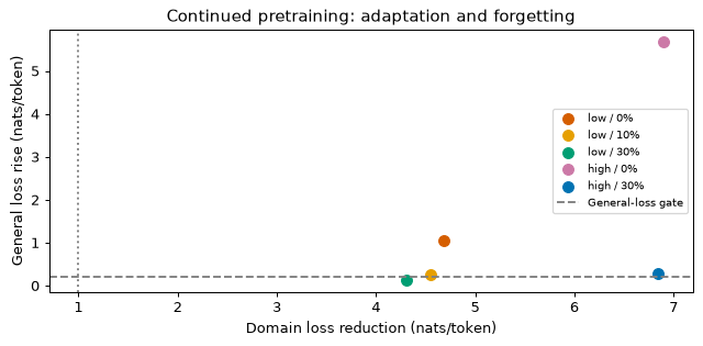
Compare the text with the quantitative test
Use the same sampling seed, temperature and token limit for every prompt/model. The small samples illustrate the kind of text produced; the held-out losses and declared gate carry the comparison. A convincing-looking safety argument can still contain invented evidence or unsupported claims.
for name in ("base","low / 0%","low / 30%"):
    for prompt,text in samples[name].items():
        print(name,"|",prompt,"|",text.replace("\n"," / "))
base | Goal G1: | Goal G1:!" /  / The squirrel was so sad. She knew that he was scared and she looked down and wanted it. He was very angry and felt sad. He decided to do the stick and it shared it up. They soon smiled and said, "Look, that!" Lila thought for a while.
base | Once upon a time | Once upon a time, there was a little girl named Tim. Timmy loved to play with her friends. /  / She wanted to work his mommy. She went to the rope and decided to do the stick. The boy was very brave and soon he was always tired. So she could have to play with a toy,
low / 0% | Goal G1: | Goal G1: The its for me shoots anarely and a safe inone seArtped. / Context CSt: The red ms end. / Gooretate magfj. / LYor The Thidries in itstose a chegetstate
low / 0% | Once upon a time | Once upon a time, there was a little girl named Tim. / Tf€� was raining, Jane looked at the garden in a zoom ugg in a clxtion accidentally string. / Gooretate Snmet: The dist soon the stles Thaigss the clrate of a safe tra
low / 30% | Goal G1: | Goal G1: The its for me shoots a loud noise and a safe in a scared day. / Goed G1: A fauggor over 1: The end. /  Everyone had a smile and a great time. He thanked the bird and helped her mom that it was hurt. /  / "
low / 30% | Once upon a time | Once upon a time, there was a little girl named Tim. Timmy loved to play with her friends. One day, she saw a big storm old boy named Lily. Timmy loved to play with her friends. One morning, they went to the frog's house,ign. Lily was so happy to find a long time
What you should see
This run’s base had general/domain losses 3.510/7.019. At the low peak, general loss rose by 1.044, 0.269 and 0.133 for 0%, 10% and 30% requested replay; domain loss ended at 2.331, 2.466 and 2.706. Only the last passed the declared gate. At the high peak, no replay raised general loss by 5.681 while reaching domain loss 0.117; 30% replay reduced that rise to 0.287 and reached 0.176, still failing the 0.20-nat limit. Actual replay shares were 10.75% and 31.0% because they were sampled. Gate decisions precede inspection of the generated examples.
The story tokenizer fragments unfamiliar engineering words. A domain-aware BPE can improve compression, but it is not interchangeable with the base’s token mapping. Continued training lowers loss on the shared domain templates; without replay, updates can raise general held-out loss. The replay/rate table shows the trade, including any conditions that fail the gate.
A stronger learning rate can adapt faster within the same step budget while moving further from the base. Replay supplies gradients for preserving the old distribution; lowering the rate limits movement. Neither guarantees retention on every capability. The losses here use one fixed tokenizer, so comparisons between checkpoints are meaningful; comparisons between different tokenizers would also need a common unit such as bits per byte.
Try this
- Sweep replay ratios with a gate declared first. Repeat seeds and evaluate separate domain templates before choosing a real adaptation recipe.
- Give the domain-only checkpoint a recovery phase on general stories, then measure both losses again. Recovery can also erase the adaptation.
- Train small BPEs on saved English/Chinese tutorial text at two language mixtures. Compare compression, keep the test text held out, and explain the embedding transition needed before an existing base could use either mapping.
Exercises
Use decimal GB and the series’ labelled compute conventions. For scaling-law questions, counts are raw parameters and tokens and the fit uses C_6=6ND. For the case-study hardware budget, include the context-dependent attention term.
Name four decisions to fix before pretraining because changing them later requires discarding work, a migration or a revised run plan. Name one decision that can change for future updates, and explain the distinction.
Show solution
The tokenizer fixes the meaning of every embedding/output row and every token in the stored shards; a new mapping requires retokenisation and an embedding transition. Model shape fixes tensor dimensions and connectivity; changing width, depth or vocabulary requires weight transfer or a new model, rather than loading the same checkpoint unchanged. Filters and deduplication fix which already-seen data influenced the weights; removing documents later does not undo those updates. A warmup-cosine horizon fixes when the rate decays; extending the run requires a deliberate new schedule, and shortening it can stop before annealing finishes.
Future data-mixture weights can change at a documented phase boundary. Batch size, checkpoint interval and parallel layout can also change with appropriate state migration. The distinction is whether a change concerns future work or invalidates an assumption about the work already completed. None of the first four makes all later change impossible; each adds a cost that belongs in the plan.
With C_6=10^{21} FLOPs and twenty tokens per parameter, calculate N, D and the loss from 1.69+406.4/N^{0.34}+410.7/D^{0.28}. Repeat for a model one quarter as large on four times the tokens. What does this buy at inference?
Show solution
Substituting D=20N gives C_6=120N^2, hence
The two reducible loss terms are 0.24684 and 0.39840, so the fitted loss is 1.69+0.24684+0.39840=2.33524 nats per token. The alternative is N'=7.2169\times10^8 and D'=2.3094\times10^{11}, with the same 6N'D'. Its terms are 0.39547 and 0.27024, giving 2.35571, worse by 0.02047 nats, or about 0.88% of the original total loss. Its predicted perplexity is about e^{0.02047}-1=2.07\% higher.
Under the approximate 2N serving charge it uses a quarter of the model arithmetic per token, and at equal weight precision a quarter of the weight storage. Attention, batching and bandwidth can change the latency relationship. Twenty tokens per parameter is a heuristic allocation; the fitted law’s own minimum at this budget is about 1.82B parameters on 91.4B tokens, loss 2.329. These fitted losses refer to the fitting distribution and tokenizer, not an assurance-task score.
A team has 64 H100s for 30 days, using the assumed dense bf16 peak of 989 TFLOP/s per GPU and 38% MFU. How many tokens fit for the exact case-study shape at context 8,192? Use N=9{,}550{,}729{,}216, N_{\text{matmul}}=8{,}927{,}875{,}072, L=36, d=4096 and 6N_{\text{matmul}}+6LTd FLOPs per token. What schedule error would the 6N shortcut cause?
Show solution
Available model compute is
The weight term is 6N_{\text{matmul}}=53{,}567{,}250{,}432 and the attention term 6(36)(8192)(4096)=7{,}247{,}757{,}312 FLOPs per token. Total: 60,815,007,744. Dividing gives D=1.02514\times10^{12} tokens, or 107.34 tokens per parameter, about half the 2T-token plan.
The shortcut gives D_6=C/(6N)=1.08795\times10^{12}, about 6.13% too many tokens. Training that many at the assumed sustained rate would take 31.84 days. A cosine schedule planned to finish at D_6 would therefore be stopped before its final decay point at day 30. Plan against the architecture-aware count, then monitor actual throughput, downtime and completed tokens.
Derive ideal MinHash-LSH candidate probability for b bands of r rows. Using at most 128 hashes, find all integer choices that catch J\ge0.85 with probability at least 0.95 and propose J\le0.5 with probability at most 0.05. Which uses the fewest hashes?
Show solution
An ideal independent MinHash row agrees with probability J. All r rows in one band agree with probability J^r. Independence across disjoint bands gives no matching band with probability (1-J^r)^b, so
This is increasing in J, so it suffices to check the two boundary similarities. Enumerate the finite integer search space:
def probability(J,b,r):
    return 1-(1-J**r)**b

feasible = [(b,r) for r in range(1,129) for b in range(1,129//r+1)
            if probability(.85,b,r)>=.95 and probability(.5,b,r)<=.05]
print(feasible)
print("Fewest hashes:",min(feasible,key=lambda pair:pair[0]*pair[1]))
The feasible pairs are (10,8),(11,8),(12,8),(13,8),(12,9),(13,9),(14,9). The smallest signature has 80 values: b=10,r=8, with probabilities 0.95847 at 0.85 and 0.03838 at 0.5. If the low-similarity limit becomes 0.6, the same search returns no feasible pair within 128 hashes. This result is an ideal probability statement, not a guarantee for every pair under the approximate universal-hash implementation of Lab 1.
C4’s cleaning discarded pages containing a curly bracket. Why does that remove much source code, and how should a corpus intended to teach code handle it?
Show solution
Braces occur in block syntax, JSON, CSS and templates, so an indiscriminate rule removes useful code alongside web scripting and boilerplate. Keep code as a separately curated source: check provenance and licences, file types, generated and minified files, lengths, secrets and duplicates using rules suitable for repositories. Choose its mixture weight explicitly. Audit code loss and tasks after changing the pipeline; an English-prose filter is not automatically a code-quality filter. Some languages use indentation instead of braces, so the rule also creates a language-dependent selection bias.
A 2T-token run gives a 15B-token mathematics source a 3% share. How often is that source seen? What changes if its weight doubles, and what three alternatives could increase mathematics exposure?
Show solution
The source contributes 0.03(2\times10^{12})=60B tokens, four times its 15B size. Doubling the share gives 120B tokens, or eight epochs. Muennighoff et al.'s data-constrained experiments found diminishing value from additional repeated data, with early repetitions more useful than later ones. Four epochs is a rough experimental regime, not a universal threshold at which learning stops. Eight exposures do not supply eight times the independent information and can increase memorisation.
Obtain more distinct mathematical text with compatible rights and provenance; generate additional problems whose solutions are checked; or concentrate the extra share in a shorter later phase so that the total additional repetitions are limited. Related code and scientific sources are another possible source of transfer. Measure held-out mathematics loss and task performance, and keep problem families out of both training and evaluation.
Show that adding a common constant to logits leaves cross-entropy unchanged. Derive the gradient of \lambda(\log Z)^2 and explain why it can help numerical stability. Does every bf16 run necessarily need this auxiliary loss?
Show solution
For a target y, cross-entropy is -z_y+\log\sum_j e^{z_j}. Replacing every z_j with z_j+c produces -(z_y+c)+c+\log\sum_j e^{z_j}, leaving the same loss and probabilities. This symmetry does not fix the common logit level. Because \partial\log Z/\partial z_j=p_j,
For positive \log Z, gradient descent pulls the normaliser down; a negative value reverses that pull. In bf16, spacing grows with magnitude: near 30 it is 0.125, so shifted logits can lose meaningful small differences. Stable log-sum-exp avoids directly overflowing exponentials, but it cannot recover differences already rounded away. Z-loss targets this drift. It is a recipe choice to test, not a requirement of all bf16 training, and it does not bound attention logits inside the model.
Starting from \Delta\mathcal L_{\text{opt}}(B)=\Delta\mathcal L_{\max}/ (1+B_{\text{noise}}/B), derive the step/token trade-off for reaching a fixed loss. Evaluate S/S_{\min} and D/D_{\min} at batches 1M and 6M tokens when B_{\text{noise}}=3M tokens.
Show solution
If the optimal progress per step is smaller by the given factor, the number of steps is S=S_{\min}(1+B_{\text{noise}}/B). Tokens are D=SB, hence D=S_{\min}(B+B_{\text{noise}}). Taking the small-batch limit defines D_{\min}=S_{\min}B_{\text{noise}}, and therefore
At 1M, the step ratio is 1+3/1=4 and the token ratio 1+1/3=1.333. At 6M they are 1+3/6=1.5 and 1+6/3=3. Larger batches use fewer updates but more tokens under this local model. Wall-clock benefit also depends on hardware utilisation, communication and the allowed learning rate; the noise scale can change during training.
For the Llama 3 8B shape, use N=8{,}030{,}261{,}248, L=32, d=4096, h_{\text{kv}}=1024, d_{\text{ff}}=14336, V=128256. On eight 80 GB GPUs, each with one 8,192-token sequence, calculate DP/ZeRO model states, activations with and without full checkpointing, and fp32 logits. Which estimated totals fit?
Show solution
Under the stated 16-byte Adam accounting, states are 16N, 4N+12N/8, 2N+14N/8 and 16N/8. Per-token-per-layer saved activations are 12(4096)+4(1024)+6(14336)=139264 bytes. Multiplying by 8192(32) gives 36.508 GB. Full checkpointing stores 2dTL=2.147 GB of layer inputs and needs 139264(8192)=1.141 GB for one recomputed layer, total 3.288 GB. Fp32 logits take 4TV=4.203 GB.
| Layout | States (GB) | Total without checkpointing | Total with checkpointing |
|---|---|---|---|
| DP | 128.484 | 169.194 | 135.975 |
| ZeRO-1 | 44.166 | 84.876 | 51.657 |
| ZeRO-2 | 30.113 | 70.823 | 37.605 |
| ZeRO-3 | 16.061 | 56.770 | 23.552 |
ZeRO-2 and ZeRO-3 pass the simplified 80 GB bound without checkpointing; all three stages pass with it. DP fails either way. Runtime buffers, communication and a memory allowance can invalidate a close fit. The case study’s wider FFN and larger parameter/vocabulary counts put ZeRO-2 at about 83.7 GB without checkpointing, above the bound. A sharding stage’s name alone does not determine whether a particular model fits.
A GPipe schedule spends one third of its wall time in its idealised pipeline bubble. Give three changes that shrink the bubble and their costs.
Show solution
Increase micro-batches m: the idle fraction (p-1)/(m+p-1) falls, but smaller micro-batches can reduce kernel efficiency, and increasing the global batch can exceed its useful noise scale. GPipe also holds many activations until backward; 1F1B reduces that memory burden. Interleave virtual stages: the idealised bubble shrinks with the number of virtual stages, at the cost of more messages and scheduling complexity. Reduce physical stages p: each GPU must hold and compute more layers, so recover memory through sharding, checkpointing or tensor parallelism. These formulas assume balanced stages; fix a slow stage before expecting a scheduling change to deliver its ideal benefit.
Training loss has a sawtooth with exactly a 1,000-step period, absent from the logged learning-rate schedule. Give two plausible causes and cheap checks.
Show solution
First, an ordered loader may cycle through differently distributed shards.
Log shard id, offset, source, document length and sampling position, then align
the loss with the cycle. Shuffle across shards or randomise their order to test
the explanation. Second, a periodic evaluation or checkpoint action may change
training state: leaving model.eval() active, consuming the training generator,
or resetting a loader. Log model.training, sampler state hashes and offsets
immediately before/after the periodic action; run it once outside the scheduled
step as a control. These are hypotheses, not a diagnosis from the loss plot
alone. Check that the logged rate is the rate actually applied to every group.
Checkpoint writes take two minutes. Explain why a fixed interval of 5,000 steps ignores the failure rate. Under Young’s approximation, how does the optimal interval change if the cluster grows tenfold and failures scale with GPU count? What does asynchronous checkpointing change?
Show solution
For a blocking write time \delta, interval \tau and mean time between job failures M, fractional overhead is approximately
The first term is writing time; the second is the average half-interval of lost work per failure. Differentiating gives -\delta/\tau^2+1/(2M)=0, or \tau^*=\sqrt{2\delta M}. Use elapsed time, not a step count whose duration may change. If M'=M/10, then \tau'^*=\tau^*/\sqrt{10}, about 0.316 of the old interval. At the optimum H^*=\sqrt{2\delta/M}, so minimum overhead grows by \sqrt{10}.
An asynchronous writer can reduce the blocking part of \delta, shortening the preferred interval. Its state copy must be consistent, and recovery can use only the latest fully durable checkpoint. Background write latency, bandwidth contention and failures while a write is pending still belong in the operational model; substituting host-copy time is only a first approximation.
Starting at 0.5, add 10^{-3} to a bf16 weight. Repeat with 3\times10^{-3}. What happens after ten successive 10^{-3} additions directly to bf16, and after ten fp32 master-weight additions followed by a bf16 copy?
Show solution
In [0.5,1), spacing is 0.5(2^{-7})=2^{-8}=0.00390625, with half-spacing 0.001953125. Thus 0.501 rounds to 0.5, while 0.503 rounds to 0.50390625. Ten separate small additions each vanish from the bf16 value, leaving 0.5. The fp32 master accumulates approximately 0.510000, whose bf16 copy is 0.51171875. Its error is within half a bf16 spacing, while direct bf16 accumulation lost the entire intended update. Verify with actual tensor arithmetic:
import torch
weight = torch.tensor(.5,dtype=torch.bfloat16)
master = torch.tensor(.5,dtype=torch.float32)
print(float(weight+.001),float(weight+.003))
for _ in range(10):
    weight += .001
    master += .001
print(float(weight),float(master),float(master.to(torch.bfloat16)))
For a subtractive update, spacing changes below the binade boundary at 0.5; the exercise specifies addition to avoid that different rounding calculation. Fp32 updates/master weights address the accumulation error. Other designs can use stochastic rounding or compensation, but require their own verification.
Continued pretraining lowers domain perplexity by 20% but raises general loss by 0.15 nats and costs three points on a general benchmark battery. Give two recipe changes, their expected effects and the acceptance decision.
Show solution
Increase general replay: more general gradients should reduce forgetting, while the same total token budget supplies fewer domain tokens and can reduce the domain gain. Lower the peak rate or shorten the run: less weight movement should limit general degradation, but can slow adaptation. These are hypotheses to check with both held-out distributions and the task battery; benchmark changes need paired uncertainty estimates.
Compare results with limits declared before the run. A 20% perplexity reduction is -\log(0.8)=0.2231 nats of domain improvement, using the same tokenizer. It does not justify accepting the three-point cost if the general gate forbids it. If no recipe passes, keep the original checkpoint and consider a narrower adaptation method or task-specific SFT in Module 09.
At laptop scale, (a) log fixed-batch validation every 25 steps of the full Lab 2 run, fit \mathcal L(D)=\mathcal L_\infty+aD^{-\gamma} on its first half, and compare the final prediction with the measured loss. (b) Run two QUICK controls, one clean and one sampling 10% of windows from a fixed 5,000-token training slice. Compare validation and slice losses. Computer runtime is additional to the exercise’s working time.
Show solution
For (a), set Lab 2’s QUICK = False and change its validation trigger from
every 150 to every 25 steps. Keep its twenty fixed batches and dedicated training
sampler; run the whole lab and preserve lab2-metrics.json. For (b), repeat
Lab 2’s setup through its model/configuration declarations in a fresh process.
The loop below uses five fixed validation batches for both QUICK controls.
Both controls begin with the same initial seed and draw the same
candidate windows; the duplicate condition alone substitutes some of them.
The fixed slice is training data, so its loss measures repeated-text fitting,
not held-out generalisation. The duplicate fraction is a Bernoulli draw per
sequence, with its actual value printed.
from scipy.optimize import least_squares

def experiment(total_steps,duplicate_share=0.0):
    torch.manual_seed(0)
    model = GPT(**config).to(device)
    optimizer = make_optimizer(model,3e-3)
    sampler = torch.Generator().manual_seed(0)
    vg = torch.Generator().manual_seed(123)
    fixed_valid = [batch(valid_data,vg,T) for _ in range(5)]
    sg = torch.Generator().manual_seed(456)
    fixed_slice = [batch(train_data[:5000],sg,T) for _ in range(5)]
    rows,duplicates = [],0
    warmup = 60 if total_steps==600 else 30
    for step in range(total_steps):
        x,y = batch(train_data,sampler,T)
        sx,sy = batch(train_data[:5000],sampler,T)
        mask = torch.rand(16,generator=sampler)<duplicate_share
        duplicates += mask.sum().item()
        x = torch.where(mask[:,None].to(device),sx,x)
        y = torch.where(mask[:,None].to(device),sy,y)
        for group in optimizer.param_groups:
            group["lr"] = learning_rate(step,total_steps,warmup,3e-3)
        optimizer.zero_grad(set_to_none=True)
        with precision():
            logits = model(x)
            loss = F.cross_entropy(logits.float().flatten(0,1),y.flatten())
        loss.backward()
        nn.utils.clip_grad_norm_(model.parameters(),1)
        optimizer.step()
        if (step+1)%25==0:
            rows.append(((step+1)*16*T,evaluate(model,fixed_valid)))
    result = dict(curve=rows,validation=evaluate(model,fixed_valid),
                  slice_loss=evaluate(model,fixed_slice),
                  duplicate_share=duplicates/(16*total_steps))
    print(total_steps,duplicate_share,result["validation"],
          result["slice_loss"],result["duplicate_share"])
    return result

# Point this to the FULL metrics saved in (a), in that run's working directory.
full = json.loads(Path("lab2-metrics.json").read_text(encoding="utf8"))
assert not full["quick"] and len(full["validation"]) >= 24
clean = experiment(150)
duplicated = experiment(150,.10)
curve = np.array([(row["tokens"],row["loss"]) for row in full["validation"]])
early = curve[curve[:,0]<=300*16*T]
scale = 1e6

def law(tokens,parameters):
    floor,amplitude,gamma = parameters
    return floor+amplitude*(tokens/scale)**(-gamma)

starts = [[floor,amplitude,gamma] for floor in (0,1,2)
          for amplitude in (1,3,10) for gamma in (.1,.5,1)]
fits = [least_squares(lambda p:law(early[:,0],p)-early[:,1],start,
                      bounds=([0,0,.001],[early[:,1].min(),100,3]))
        for start in starts]
fit = min(fits,key=lambda result:np.sum(result.fun**2))
prediction = law(curve[-1,0],fit.x)
print("Fitted parameters:",fit.x)
print("Final prediction, measurement, error:",prediction,curve[-1,1],
      prediction-curve[-1,1])
fig,ax = plt.subplots(figsize=(7.2,3.6))
ax.loglog(curve[:,0],curve[:,1],"o",label="Measured validation")
ax.loglog(curve[:,0],law(curve[:,0],fit.x),label="First-half fit extrapolated")
ax.axvline(300*16*T,color="gray",linestyle="--",label="Fitting boundary")
ax.set(xlabel="Training tokens seen",ylabel="Cross-entropy (nats/token)")
ax.legend()
plt.show()
Fit only the early measurements before inspecting the end. Report the error, not a promised accuracy: a short curve can poorly identify its floor/exponent, and cosine annealing changes the late trajectory. A stable-rate phase gives a cleaner token-scaling comparison. The constrained multi-start fit above makes the fitting assumptions visible; it is not an uncertainty interval.
In this environment the standard FULL curve’s first-half fit predicted 2.9551 against measured 2.8327, an error of +0.1224 nats. The fitted floor, amplitude at one million tokens and exponent were 2.1897, 1.1679 and 0.4700. The two QUICK controls measured:
| Control | Actual duplicate share | Held-out loss | Fixed training-slice loss |
|---|---|---|---|
| Clean | 0% | 3.7984 | 3.8140 |
| Duplicated | 9.958% | 4.3431 | 4.0267 |
The repeated slice has a 0.3164-nat advantage over validation in the duplicate run, while the clean run’s two losses are similar. Its absolute slice loss is still higher than in the clean run: repetition did not improve every measure. Held-out loss worsened by 0.5447 nats in this seed. These controls consume the sampler differently from Lab 2’s ordinary loop and use five rather than twenty evaluation batches, so their numbers should be compared with each other.
In the duplicate comparison, look for slice loss falling more than general validation. A 150-step run consumes 614,400 tokens, so 10% replay of a 5,000-token slice is about 12.3 token-equivalent exposures, with overlapping windows rather than twelve literal sequential passes. Validation may improve or worsen within run/measurement noise; repeating seeds is required before attributing a small change to duplication. Record the actual fraction and compare the clean run’s slice loss too: common story patterns can be easy even without deliberate replay.
Self-check quiz
Choose one answer per question. Review the explanation after committing to an answer; the wrong options represent different accounting mistakes.
Guided reading
Read for the experimental comparison and accounting assumptions. Reproduce one result or calculation before accepting the proposed recipe.
Why read it. A documented web-data pipeline with ablations of filtering and deduplication, including decisions whose first version did not improve the resulting model.
What to read. Read the introduction, the sections on text extraction, base filtering, deduplication (including the per-snapshot finding) and the FineWeb-Edu annotation and classifier. Skim the custom heuristic filters and the comparison with other datasets. Skip the appendices.
Questions to answer while reading.
- Why did the authors extract text from WARC files with trafilatura instead of using the WET text, and how did they show that it mattered?
- What went wrong when they deduplicated across all crawl snapshots at once, and what did they do instead? Why might global deduplication favour older, lower-quality text?
- How was the educational-quality classifier built (annotator, scale, number of annotated samples, model) and what threshold produced FineWeb-Edu?
- What size of model and how many tokens did they use for their data ablations, and what does that imply about how data decisions are tested?
Why read it. The source of the 16-bytes-per-parameter accounting and of the three sharding stages that s8 and s9 derive and that FSDP implements.
What to read. Read the introduction with its memory figure, the analysis of where the memory goes (model states and residual states), the description of the three ZeRO-DP stages, and the communication analysis. Skim ZeRO-R. Skip the implementation and evaluation sections.
Questions to answer while reading.
- Reproduce the paper’s per-GPU memory for a 7.5B-parameter model on 64 GPUs under the baseline and the three stages (120, 31.4, 16.6 and 1.9 GB).
- Why does sharding the parameters cost only 1.5 times data parallelism’s communication rather than more?
- What are ‘residual states’, and which techniques in this module address each of them?
Why read it. Shows that the instabilities of large runs can be reproduced and fixed in small models at high learning rates: the method Lab 3 copies, and the evidence behind QK-norm, z-loss and the AdamW epsilon advice.
What to read. Read the introduction, the sections on attention-logit growth with qk-layernorm and on output-logit divergence with z-loss, and the definition of learning-rate sensitivity. Skim the section on other interventions (warmup, independent weight decay, muParam, the AdamW epsilon). Skip the appendices.
Questions to answer while reading.
- What is learning-rate sensitivity and why is it a more useful summary than the best loss achieved?
- What evidence links attention-logit growth to divergence, and how does qk-layernorm change the sensitivity curve? Compare with what Lab 3 measured.
- Why does z-loss fix output-logit divergence, and what happens to the logits without it?
- What do the authors find about AdamW’s epsilon as models grow, and what do they recommend?
Summary
- Fix tokenizer, shape, data policy and run horizon before paying for the main run; record every later phase change.
- Training compute includes the matrix weights and context-dependent attention; use the same convention when planning tokens, time and MFU.
- Data cleaning is a policy with false positives, and every removed document should have an auditable reason.
- Exact fingerprints, MinHash-LSH candidate generation and exact overlap verification answer different duplicate questions.
- Mixture weights determine source exposure; repeated tokens supply diminishing new information and can encourage memorisation.
- Packing saves padding but requires a deliberate policy on EOS boundaries, document attention and validation splits.
- Learning-rate schedules, batch size and optimiser moments affect the trajectory, so monitor the rate and pre-clipping gradients actually used.
- Diagnose attention-logit growth and output-logit drift separately; clipping, QK norms and z-loss act on different quantities.
- Count model states, saved activations, logits and runtime allowances before selecting sharding, checkpointing or parallelism.
- Checkpoints must restore optimiser and sampler state for resumption, and only fully written checkpoints are recoverable.
- Evaluate fixed held-out distributions and paired task outcomes; a lower training loss or a small aggregate benchmark gain alone is insufficient.
- Continued pretraining trades domain adaptation against retention, and its acceptance gate must be declared before inspecting the results.
The kept base checkpoint is a distribution modeller. Module 09 turns it towards instructed behaviour through supervised fine-tuning and preference training. The case-study team carries forward its continued-pretraining checkpoint only if the domain and general gates pass; otherwise it keeps the released checkpoint.
Key terms
| English | 中文 |
|---|---|
| pretraining, base model | 预训练,基座模型 |
| compute budget | 算力预算 |
| model FLOPs utilisation (MFU) | 模型算力利用率 |
| compute-optimal, over-training | 计算最优,过度训练 |
| corpus, data mixture | 语料,数据配比 |
| quality filter | 质量过滤器 |
| language identification | 语种识别 |
| deduplication, near-duplicate | 去重,近似重复 |
| MinHash, locality-sensitive hashing (LSH) | 最小哈希,局部敏感哈希 |
| contamination, decontamination | 数据污染,去污染 |
| tokenizer training | 分词器训练 |
| sequence packing | 序列打包 |
| mixture of experts, expert parallelism | 混合专家,专家并行 |
| load balancing, capacity factor | 负载均衡,容量因子 |
| warmup, cosine decay | 预热,余弦衰减 |
| warmup-stable-decay (WSD) schedule | 预热-稳定-衰减(WSD)调度 |
| critical batch size | 临界 batch 大小 |
| gradient clipping | 梯度裁剪 |
| mixed precision (bf16), loss scaling | 混合精度(bf16),损失缩放 |
| loss spike, divergence | 损失尖峰,发散 |
| activation checkpointing (gradient checkpointing) | 激活检查点(梯度检查点) |
| data / tensor / pipeline parallelism | 数据 / 张量 / 流水线并行 |
| sequence / context parallelism | 序列并行 / 上下文并行 |
| ZeRO, fully sharded data parallel (FSDP) | 零冗余优化器,全分片数据并行 |
| all-reduce | 全归约 |
| pipeline bubble | 流水线气泡 |
| silent data corruption | 静默数据损坏 |
| mid-training, context extension | 中期训练,上下文扩展 |
| continued pretraining, replay | 继续预训练,回放 |
| catastrophic forgetting | 灾难性遗忘 |
References
- Hoffmann, J. et al. “Training compute-optimal large language models.” NeurIPS, 2022. Chinchilla: the L(N, D) fit and the 20-tokens-per-parameter rule used in s1.
- Kaplan, J. et al. “Scaling laws for neural language models.” arXiv, 2020. The 6N-per-token approximation and the insensitivity of loss to model shape at fixed N.
- Besiroglu, T., Erdil, E., Barnett, M., You, J. “Chinchilla scaling: A replication attempt.” arXiv, 2024. Re-analysis of the Chinchilla parametric fit.
- Rae, J. W. et al. “Scaling language models: Methods, analysis and insights from training Gopher.” arXiv, 2021. The Gopher quality and repetition filters.
- Raffel, C. et al. “Exploring the limits of transfer learning with a unified text-to-text transformer.” JMLR, 2020. C4 and its line-level cleaning rules.
- Dodge, J. et al. “Documenting large webtext corpora: A case study on the Colossal Clean Crawled Corpus.” EMNLP, 2021. What C4’s blocklist removed, and from whom.
- Penedo, G. et al. “The FineWeb datasets: Decanting the web for the finest text data at scale.” NeurIPS Datasets and Benchmarks Track, 2024. A documented public web pipeline and FineWeb-Edu.
- Li, J. et al. “DataComp-LM: In search of the next generation of training sets for language models.” NeurIPS Datasets and Benchmarks Track, 2024. DCLM and its fastText quality classifier.
- Barbaresi, A. “Trafilatura: A web scraping library and command-line tool for text discovery and extraction.” ACL System Demonstrations, 2021. Boilerplate removal.
- Joulin, A., Grave, E., Bojanowski, P., Mikolov, T. “Bag of tricks for efficient text classification.” EACL, 2017. fastText, the basis of common language-identification models.
- Broder, A. Z. “On the resemblance and containment of documents.” Compression and Complexity of Sequences, 1997. MinHash.
- Leskovec, J., Rajaraman, A., Ullman, J. D. Mining of Massive Datasets, Chapter 3. Cambridge University Press. Shingling, MinHash and LSH banding with the S-curve.
- Lee, K. et al. “Deduplicating training data makes language models better.” ACL, 2022.
- Hernandez, D. et al. “Scaling laws and interpretability of learning from repeated data.” arXiv, 2022. The cost of a small fraction of heavily repeated data.
- Brown, T. et al. “Language models are few-shot learners.” NeurIPS, 2020. GPT-3; 13-gram decontamination.
- Muennighoff, N. et al. “Scaling data-constrained language models.” NeurIPS, 2023. How much repeated data is worth.
- Xie, S. M. et al. “DoReMi: Optimizing data mixtures speeds up language model pretraining.” NeurIPS, 2023. Learned mixture weights.
- Xue, L. et al. “mT5: A massively multilingual pre-trained text-to-text transformer.” NAACL, 2021. Temperature sampling of languages.
- Ding, H. et al. “Fewer truncations improve language modeling.” ICML, 2024. Best-fit packing.
- Eldan, R., Li, Y. “TinyStories: How small can language models be and still speak coherent English?” arXiv, 2023. The dataset of Labs 1, 2, 3 and 5.
- Touvron, H. et al. “Llama 2: Open foundation and fine-tuned chat models.” arXiv, 2023. A published recipe: learning rates, schedule, batch, clipping.
- Grattafiori, A. et al. “The Llama 3 herd of models.” arXiv, 2024. Annealing, context extension, document masking and interruption statistics at scale.
- Chowdhery, A. et al. “PaLM: Scaling language modeling with Pathways.” JMLR, 2023. Rewind-and-skip for loss spikes; the MFU definition.
- Fedus, W., Zoph, B., Shazeer, N. “Switch Transformers: Scaling to trillion parameter models with simple and efficient sparsity.” JMLR, 2022. Load-balancing loss and capacity factor.
- Lepikhin, D. et al. “GShard: Scaling giant models with conditional computation and automatic sharding.” ICLR, 2021. Expert parallelism.
- Jiang, A. Q. et al. “Mixtral of experts.” arXiv, 2024.
- Dai, D. et al. “DeepSeekMoE: Towards ultimate expert specialization in mixture-of-experts language models.” ACL, 2024. Fine-grained and shared experts.
- DeepSeek-AI. “DeepSeek-V3 technical report.” arXiv, 2024. Auxiliary-loss-free load balancing; FP8 training with fine-grained scaling.
- DeepSeek-AI. “DeepSeek LLM: Scaling open-source language models with longtermism.” arXiv, 2024. Fitted scaling of learning rate and batch size with compute.
- Yang, G. et al. “Tensor Programs V: Tuning large neural networks via zero-shot hyperparameter transfer.” NeurIPS, 2021. muP.
- Loshchilov, I., Hutter, F. “Decoupled weight decay regularization.” ICLR, 2019. AdamW.
- McCandlish, S., Kaplan, J., Amodei, D. et al. “An empirical model of large-batch training.” arXiv, 2018. The gradient noise scale and the critical batch size.
- Hägele, A. et al. “Scaling laws and compute-optimal training beyond fixed training durations.” NeurIPS, 2024. Warmup-stable-decay against cosine.
- Hu, S. et al. “MiniCPM: Unveiling the potential of small language models with scalable training strategies.” arXiv, 2024. The WSD schedule.
- Micikevicius, P. et al. “Mixed precision training.” ICLR, 2018. Loss scaling and fp32 master weights.
- Micikevicius, P. et al. “FP8 formats for deep learning.” arXiv, 2022. E4M3 and E5M2.
- Dehghani, M. et al. “Scaling vision transformers to 22 billion parameters.” ICML, 2023. QK normalisation against attention-logit growth.
- Wortsman, M. et al. “Small-scale proxies for large-scale Transformer training instabilities.” ICLR, 2024. Instabilities reproduced at small scale; QK-norm, z-loss, AdamW epsilon.
- Chen, T., Xu, B., Zhang, C., Guestrin, C. “Training deep nets with sublinear memory cost.” arXiv, 2016. Activation (gradient) checkpointing.
- Korthikanti, V. et al. “Reducing activation recomputation in large transformer models.” MLSys, 2023. The activation-memory count, sequence parallelism, selective recomputation.
- Dao, T. et al. “FlashAttention: Fast and memory-efficient exact attention with IO-awareness.” NeurIPS, 2022.
- Rajbhandari, S., Rasley, J., Ruwase, O., He, Y. “ZeRO: Memory optimizations toward training trillion parameter models.” SC, 2020.
- Zhao, Y. et al. “PyTorch FSDP: Experiences on scaling fully sharded data parallel.” VLDB, 2023.
- Shoeybi, M. et al. “Megatron-LM: Training multi-billion parameter language models using model parallelism.” arXiv, 2019. Tensor parallelism.
- Narayanan, D. et al. “Efficient large-scale language model training on GPU clusters using Megatron-LM.” SC, 2021. Interleaved pipeline schedules and 3D parallelism.
- Huang, Y. et al. “GPipe: Efficient training of giant neural networks using pipeline parallelism.” NeurIPS, 2019.
- Liu, H., Zaharia, M., Abbeel, P. “Ring attention with blockwise transformers for near-infinite context.” ICLR, 2024. Context parallelism.
- Jacobs, S. A. et al. “DeepSpeed Ulysses: System optimizations for enabling training of extreme long sequence Transformer models.” arXiv, 2023.
- Young, J. W. “A first order approximation to the optimum checkpoint interval.” Communications of the ACM, 1974.
- Dixit, H. D. et al. “Silent data corruptions at scale.” arXiv, 2021.
- Chen, S. et al. “Extending context window of large language models via positional interpolation.” arXiv, 2023.
- Peng, B. et al. “YaRN: Efficient context window extension of large language models.” ICLR, 2024.
- Gururangan, S. et al. “Don’t stop pretraining: Adapt language models to domains and tasks.” ACL, 2020. Domain- and task-adaptive continued pretraining.
- Gupta, K. et al. “Continual pre-training of large language models: How to (re)warm your model?” arXiv, 2023.
- Ibrahim, A. et al. “Simple and scalable strategies to continually pre-train large language models.” TMLR, 2024. Re-warming, re-decaying and replay.