The learning problem
An engineer has a function in mind and cannot write it down. The sag of a scaffold as a function of its material and geometry can be computed by a solver, but the solver took a person-year to build. The probability that a hazard is controllable, as a function of the situation, cannot be computed at all; it is estimated by people. Machine learning is the practice of obtaining such a function from examples of its inputs and outputs, when the examples are cheaper than the theory.
Formally, there is an unknown function f^\ast and a data distribution P over pairs (\mathbf{x}, y) of inputs \mathbf{x} \in \R^d and outputs y. The function f^\ast is the best possible prediction of y from \mathbf{x}; the outputs scatter around it because the inputs do not determine them completely. We see a sample \mathcal{D} = \{(\mathbf{x}_i, y_i)\}_{i=1}^{N} drawn from P, and we want a function f that predicts y from \mathbf{x} well on inputs we have not seen. The last clause is the whole subject. Predicting the examples we already have is a lookup table.
Expected risk and empirical risk
A loss \ell(f(\mathbf{x}), y) \ge 0 says how wrong one prediction is, for example the squared error (f(\mathbf{x}) - y)^2. What we want small is the expected risk, the average loss over the distribution the inputs will come from:
It cannot be computed, because P is unknown. What can be computed, for a model f_\theta with parameters \theta, is the empirical risk, the average loss over the sample:
For parameters fixed before the sample is drawn, \mathcal{L}(\theta) is an unbiased estimate of R(f_\theta): each term has expectation R(f_\theta). Fitting destroys that property. The optimiser chooses \hat\theta to make \mathcal{L} small on these N examples, noise included, so the training loss at \hat\theta is biased low. For an optimiser that finds the minimum the argument takes three steps. Write R(\theta) for R(f_\theta) and let \theta^\circ minimise it over the model family. Then \mathcal{L}(\hat\theta) \le \mathcal{L}(\theta^\circ) for every sample, because \hat\theta minimises \mathcal{L}; \E[\mathcal{L}(\theta^\circ)] = R(\theta^\circ), because \theta^\circ does not depend on the sample; and R(\theta^\circ) \le R(\hat\theta), because \theta^\circ is the best. Chained:
The gap between the training loss and the expected risk is the subject of Section 8, which measures how it grows with the flexibility of the model, and of Section 10, which estimates the expected risk without fooling yourself.
Three settings
- Supervised learning. y is given for every example: regression when y is continuous, classification when it is one of K labels. Most of this series.
- Unsupervised learning. No y. The task is to find structure: clusters, low-dimensional coordinates, densities. k-means and principal component analysis appear in Section 11; the neural forms are in Module 05.
- Reinforcement learning. No y either, but a reward that arrives after actions. Module 09 uses it to train language models.
The five ingredients
Every learning method, from a straight line to a language model, is specified by five choices. Write them down for any method you meet; a method you cannot state this way is one you do not understand yet.
- Data. \mathcal{D}, and the distribution P it came from. The second is the one people forget. Everything learned is learned about P, so a model is only as good as the match between P and the inputs it will meet in service.
- Model. A family of functions f_\theta indexed by parameters \theta, also called the hypothesis class. It fixes what can be learned at all: a line has two parameters and can only ever be a line; a language model has billions.
- Loss. \ell \ge 0 and its average over the data, the empirical risk \mathcal{L}(\theta). It decides which mistakes count and how much; Section 5 shows that it also states an assumption about the noise.
- Optimiser. A procedure that finds \theta making \mathcal{L} small, almost always a variant of gradient descent (Sections 3 and 4). It decides whether the \theta the loss asks for is actually found, and at what cost.
- Evaluation. A measurement of how well f_\theta does on data it was not fitted to: an estimate of R, not the loss on \mathcal{D}, which the optimiser has already minimised.
| Ingredient | This module’s linear regression | The language model of Modules 07–10 |
|---|---|---|
| Data | 200 rows, 3 features; Gaussian noise of standard deviation 0.1 | trillions of tokens of text |
| Model | \mathbf{w}^\top\mathbf{x} + b: 4 parameters | a transformer: about 9.5 billion parameters |
| Loss | squared error | cross-entropy over the vocabulary at every position |
| Optimiser | the normal equations, or gradient descent | AdamW |
| Evaluation | RMSE on held-out rows | held-out perplexity and task benchmarks |
The five slots are the same. The parameter counts differ by a factor of 9.5\times10^{9}/4 \approx 2.4\times10^{9}, more than nine orders of magnitude. The language model is the hypothetical case study that Modules 07–10 follow; nothing about it is needed before then.
| Ingredient | Neo-Hookean fit to one compression test |
|---|---|
| Data | 16 triples (stretch, stress, recorded uncertainty) from one test; the distribution is specimens of this gel tested this way |
| Model | nominal stress P = 2c_1(\lambda - \lambda^{-2}) at stretch \lambda: one parameter, c_1 |
| Loss | squared error weighted by 1/\sigma_i^2, the inverse square of each point’s uncertainty |
| Optimiser | a closed form |
| Evaluation | residuals on strain ranges held out of the fit |
The symbols P and \lambda carry these meanings only in this example and in Section 12. The evaluation slot is where Section 12’s main question lives: residuals inside the fitted strain range can be checked, while a prediction outside it is an extrapolation that no residual inside the range can vouch for.
Inputs are numbers
A model sees a feature vector \mathbf{x} \in \R^d. A measured quantity is already a number; a category, such as a material grade, a supplier or a defect type, is not. Encode a K-way category as one-hot: K binary columns, with a 1 in the column of the observed category and 0 in the others. Never code it as the integers 1, \dots, K: a linear model then treats the category as a quantity, which imposes an order and equal spacing between consecutive codes. The exception is a genuinely ordinal scale, such as a severity from minor to critical, whose order is real; even then, integer codes assume equal steps between the levels, a modelling choice to check rather than a fact.
One-hot codes also explain learned representations. A one-hot row vector \mathbf{e}_k^\top times a trainable K \times m table picks out row k of the table, so an embedding is such a table learned with the rest of the model, and it works the same way for any categorical feature (a part number, a supplier, a sensor ID) as for the tokens of a language model. Module 06, Section 4 shows the token embedding entering the transformer’s residual stream, and Module 06, Section 11 counts its V \times d table.
The running examples
Four examples recur in this module, so that each new idea lands on something already familiar:
- a synthetic linear regression with N = 200 rows and d = 3 features (Sections 2–4, Lab 1);
- noisy samples of \sin(2\pi x) fitted by polynomials (Sections 8–9, Lab 3);
- a classifier of breast tumours as malignant or benign, on the dataset that ships with scikit-learn (Sections 6–7, Labs 2 and 4);
- a hyperelastic material model fitted to a compression test of a soft hydrogel (Sections 5 and 12, Lab 5).
Why is the training loss not a measure of how good the model is?
Show answer
The optimiser chose \theta to make it small on those very examples, noise included, so it is biased low. Only data that played no part in the fitting estimate the expected risk without that bias.
A defect severity {minor, major, critical} is coded 1, 2, 3 in a linear model. What does that assume, and when is it acceptable?
Show answer
It assumes an order, which is real here, and equal steps: the effect of “major” lies exactly halfway between those of “minor” and “critical”. Keep the integer code only if equal steps are plausible or validation data support them; otherwise one-hot encode, which keeps no order and assumes no spacing. (Exercise 2 takes the unordered case.)
Least squares and its geometry
Linear regression is the simplest model that exercises every ingredient, and the only one in this module whose every property can be computed exactly. This section fits it in closed form, reads the answer as a projection, and says when the problem is ill-posed and how to compute the answer stably.
Set-up
Let f(\mathbf{x}) = \mathbf{w}^\top\mathbf{x} + b. Absorb the intercept b by appending a constant 1 to every input, so that f(\mathbf{x}) = \mathbf{w}^\top\mathbf{x} with \mathbf{w} \in \R^{d+1} and b its last entry. Stack the inputs as the rows of \mathbf{X} \in \R^{N\times(d+1)}, whose last column is all ones, and the outputs as \mathbf{y} \in \R^N. The loss is the mean squared error:
Section 5 shows why squared error is the right loss when the noise is Gaussian; here take it as given.
The gradient, derived
Expand the squared norm as an inner product:
The two cross terms \mathbf{w}^\top\mathbf{X}^\top\mathbf{y} and \mathbf{y}^\top\mathbf{X}\mathbf{w} are the same scalar, one the transpose of the other, which is where the 2 comes from. Two identities differentiate the pieces. For a symmetric matrix \mathbf{A}, \nabla_{\mathbf{w}}(\mathbf{w}^\top\mathbf{A}\mathbf{w}) = 2\mathbf{A}\mathbf{w}: writing the sum out, \partial_{w_k}\sum_{j,l}w_jA_{jl}w_l = \sum_l A_{kl}w_l + \sum_j w_jA_{jk} = 2(\mathbf{A}\mathbf{w})_k, the last step by symmetry. For a constant vector \mathbf{c}, \nabla_{\mathbf{w}}(\mathbf{c}^\top\mathbf{w}) = \mathbf{c}. With \mathbf{A} = \mathbf{X}^\top\mathbf{X} and \mathbf{c} = \mathbf{X}^\top\mathbf{y},
The gradient is the residual vector \mathbf{X}\mathbf{w} - \mathbf{y} mapped back to parameter space by \mathbf{X}^\top. Differentiating once more gives the Hessian \frac{2}{N}\mathbf{X}^\top\mathbf{X}, the same at every \mathbf{w}. It is positive semidefinite, because \mathbf{v}^\top\mathbf{X}^\top\mathbf{X}\mathbf{v} = \|\mathbf{X}\mathbf{v}\|^2 \ge 0 for every \mathbf{v}. So \mathcal{L} is a convex quadratic, and every point where its gradient vanishes is a global minimum.
The normal equations
Setting the gradient to zero gives the normal equations
If \mathbf{X} has full column rank, its d + 1 columns linearly independent, then \|\mathbf{X}\mathbf{v}\|^2 > 0 for every \mathbf{v} \ne \mathbf{0}, so \mathbf{X}^\top\mathbf{X} is positive definite and invertible, and the minimiser is unique:
Full column rank needs at least d + 1 linearly independent rows: no fewer examples than parameters. The formula is for reading; how to compute \mathbf{w}^\ast comes below.
The geometry: an orthogonal projection
As \mathbf{w} varies, \mathbf{X}\mathbf{w}, a linear combination of the columns of \mathbf{X}, sweeps out the column space of \mathbf{X}, a subspace of dimension d + 1 inside \R^N. Least squares picks the point of that subspace closest to \mathbf{y}. With the residual \mathbf{r} = \mathbf{y} - \mathbf{X}\mathbf{w}^\ast, the normal equations read
each column of \mathbf{X} has zero inner product with the residual. The residual is perpendicular, or normal, to the column space, which is where the equations get their name, and \hat{\mathbf{y}} = \mathbf{X}\mathbf{w}^\ast is the orthogonal projection of \mathbf{y} onto it: the foot of the perpendicular from \mathbf{y}, which is the closest point (Figure 1.1).
Least squares as a projection, drawn in three dimensions. A plane through the origin, spanned by two column vectors \mathbf{x}_{(1)} and \mathbf{x}_{(2)}, is the column space of \mathbf{X}. The data vector \mathbf{y} rises above the plane; its foot in the plane is \hat{\mathbf{y}} = \mathbf{X}\mathbf{w}^\ast; the residual \mathbf{r} = \mathbf{y} - \hat{\mathbf{y}} is a dashed segment that meets the plane at a right angle. \mathbf{X}^\top\mathbf{r} = \mathbf{0} are the normal equations.
The projection is linear: \hat{\mathbf{y}} = \mathbf{P}\mathbf{y} with
the hat matrix, so called because it puts the hat on \mathbf{y}. (Statistics texts write it \mathbf{H}; this module keeps \mathbf{H} for the Hessian.) It is symmetric and idempotent, \mathbf{P}^2 = \mathbf{X}(\mathbf{X}^\top\mathbf{X})^{-1}(\mathbf{X}^\top\mathbf{X})(\mathbf{X}^\top\mathbf{X})^{-1}\mathbf{X}^\top = \mathbf{P}: projecting twice changes nothing. Its trace counts the dimensions it projects onto. Using \operatorname{tr}(\mathbf{A}\mathbf{B}) = \operatorname{tr}(\mathbf{B}\mathbf{A}), \operatorname{tr}\mathbf{P} = \operatorname{tr}\big((\mathbf{X}^\top\mathbf{X})^{-1}\mathbf{X}^\top\mathbf{X}\big) = \operatorname{tr}\mathbf{I}_{d+1} = d + 1, the number of fitted parameters. Section 9 turns this count into the effective degrees of freedom of ridge regression.
Two consequences follow when \mathbf{X} contains the column of ones. That column’s row of \mathbf{X}^\top\mathbf{r} = \mathbf{0} reads \sum_i r_i = 0: the residuals sum to zero, and \hat{\mathbf{y}} has the same mean \bar y as \mathbf{y}. And because \bar y\mathbf{1} also lies in the column space, \mathbf{y} - \bar y\mathbf{1} = (\hat{\mathbf{y}} - \bar y\mathbf{1}) + \mathbf{r} splits the centred data into a part inside the column space and a part perpendicular to it. Pythagoras gives
the total sum of squares is the explained plus the residual sum of squares. It defines the coefficient of determination
the fraction of the variance of \mathbf{y} about its mean that the fit explains; on the training data it lies between 0 and 1. Predicting the mean everywhere is the model with only an intercept, so R^2 compares the fit with that baseline. Section 7 uses R^2 on held-out data, where the identity no longer holds and R^2 can be negative.
Fit y = b + wx to x = (0, 1, 2, 3) and y = (1, 3, 2, 5). The rows of \mathbf{X} are (1, x_i), so
with \sum x_iy_i = 0 + 3 + 4 + 15 = 22. The determinant is 4\cdot14 - 6\cdot6 = 20, and Cramer’s rule gives
The fitted values are \hat{\mathbf{y}} = (1.1, 2.2, 3.3, 4.4) and the residuals \mathbf{r} = (-0.1, 0.8, -1.3, 0.6). Check the normal equations: \sum r_i = -0.1 + 0.8 - 1.3 + 0.6 = 0 and \sum x_ir_i = 0 + 0.8 - 2.6 + 1.8 = 0, both exactly. The sums of squares are RSS = 0.01 + 0.64 + 1.69 + 0.36 = 2.70; with \bar y = 2.75, TSS = 1.75^2 + 0.25^2 + 0.75^2 + 2.25^2 = 8.75; and ESS = 1.65^2 + 0.55^2 + 0.55^2 + 1.65^2 = 6.05, so 6.05 + 2.70 = 8.75 as Pythagoras requires. Hence R^2 = 1 - 2.70/8.75 = 0.691. The hat matrix has diagonal (0.7, 0.3, 0.3, 0.7) and trace 2, the number of parameters.
When the columns are dependent
If one column of \mathbf{X} is a linear combination of the others, there is a
\mathbf{v} \ne \mathbf{0} with \mathbf{X}\mathbf{v} = \mathbf{0}; then
\mathbf{X}^\top\mathbf{X}\mathbf{v} = \mathbf{0}, and \mathbf{X}^\top\mathbf{X} is singular.
Two ways it happens in practice: a temperature in °C next to the same temperature in °F, with an
intercept, since T_{\text{F}} = 1.8\,T_{\text{C}} + 32 makes the °F column a combination of the
°C column and the column of ones; and all K one-hot columns of a category next to an intercept,
since the K columns sum to the column of ones. Every \mathbf{w}^\ast + t\mathbf{v} then fits
equally well. The projection \hat{\mathbf{y}} is still unique, and so are the predictions at
the training inputs and at any new input that obeys the same dependency; the weights are not.
The pseudo-inverse solution \mathbf{X}^{+}\mathbf{y} picks, among all the minimisers, the
one of smallest norm, and it is what np.linalg.lstsq returns. The ridge penalty of
Section 9 also removes the ambiguity. Neither makes the individual weights of dependent
columns meaningful.
Append a column 2x to the four points, so the rows of \mathbf{X} are (1, x_i, 2x_i) and
whose third row is twice its second: the determinant is 0. Write a and c for the weights on
x and 2x. The fit is b + (a + 2c)x, so every choice with b = 1.1 and a + 2c = 1.1
reproduces the line of the previous example and the predictions (1.1, 2.2, 3.3, 4.4). The
minimum-norm choice is the point of the line a + 2c = 1.1 closest to the origin, which lies
along the line’s normal (1, 2): (a, c) = 1.1\cdot(1, 2)/(1^2 + 2^2) = (0.22, 0.44).
np.linalg.lstsq returns (b, a, c) = (1.1, 0.22, 0.44) and reports rank 2.
Computing it
Never form (\mathbf{X}^\top\mathbf{X})^{-1}; solve. The condition number \kappa(\mathbf{X}), the ratio of the largest to the smallest singular value of \mathbf{X}, bounds how much rounding errors can be amplified: of the 16 significant digits of double precision, a solve can lose about \log_{10}\kappa. Three methods, in increasing order of robustness:
- Cholesky of \mathbf{X}^\top\mathbf{X}. Factor \mathbf{X}^\top\mathbf{X} = \mathbf{L}\mathbf{L}^\top with \mathbf{L} lower-triangular and solve two triangular systems. It is the fastest, but forming \mathbf{X}^\top\mathbf{X} squares the condition number, \kappa(\mathbf{X}^\top\mathbf{X}) = \kappa(\mathbf{X})^2, because the eigenvalues of \mathbf{X}^\top\mathbf{X} are the squared singular values of \mathbf{X}. At \kappa(\mathbf{X}) = 10^6 that is up to 12 lost digits instead of 6.
- QR of \mathbf{X}. Write \mathbf{X} = \mathbf{Q}\mathbf{R}, with orthonormal columns in \mathbf{Q} and \mathbf{R} upper-triangular. Since \mathbf{Q}^\top\mathbf{Q} = \mathbf{I}, the normal equations become \mathbf{R}^\top\mathbf{R}\mathbf{w} = \mathbf{R}^\top\mathbf{Q}^\top\mathbf{y}, that is \mathbf{R}\mathbf{w} = \mathbf{Q}^\top\mathbf{y}, solved by back-substitution. The method works with \mathbf{X} itself and never squares \kappa.
- SVD. \mathbf{X} = \mathbf{U}\boldsymbol{\Sigma}\mathbf{V}^\top gives \mathbf{w} = \mathbf{V}\boldsymbol{\Sigma}^{-1}\mathbf{U}^\top\mathbf{y}. The singular values on the diagonal of \boldsymbol{\Sigma} display the conditioning, and inverting only the non-zero ones gives the minimum-norm solution of the rank-deficient case.
np.linalg.lstsq uses an SVD-based LAPACK driver and is the default to reach for. Each method
costs about Nd^2 operations to form \mathbf{X}^\top\mathbf{X} or to factor \mathbf{X}, plus
about d^3 for the small solve that follows.
The code, and the irreducible error
Here is all of it in NumPy, on the data of Lab 1: 200 inputs with three standard-normal features, true weights (1.5, -2.0, 0.5), intercept 0.7 and Gaussian noise of standard deviation 0.1. Gradient descent, the subject of the next section, is included for comparison.
import numpy as np

rng = np.random.default_rng(0)
N, d = 200, 3
X = rng.normal(size=(N, d))
w_true = np.array([1.5, -2.0, 0.5]); b_true = 0.7
y = X @ w_true + b_true + 0.1 * rng.normal(size=N)   # noise: the part no model recovers

Xb = np.hstack([X, np.ones((N, 1))])                 # absorb the bias

# closed form
w_closed = np.linalg.solve(Xb.T @ Xb, Xb.T @ y)

# gradient descent
w = np.zeros(d + 1); eta = 0.1
for step in range(500):
    grad = (2 / N) * Xb.T @ (Xb @ w - y)
    w -= eta * grad
print(np.round(w_closed, 3), np.round(w, 3))         # both near [1.5, -2.0, 0.5, 0.7]

# the robust default: an SVD-based solver that never forms Xb.T @ Xb
w_lstsq = np.linalg.lstsq(Xb, y, rcond=None)[0]
rss = np.sum((y - Xb @ w_lstsq) ** 2)               # residual sum of squares
print(np.round(w_lstsq, 3))
print(f"residual RMS {np.sqrt(rss / N):.4f}")
print(f"sqrt(RSS / (N - 4)) {np.sqrt(rss / (N - 4)):.4f}")
[ 1.491 -2.01   0.505  0.696] [ 1.491 -2.01   0.505  0.696]
[ 1.491 -2.01   0.505  0.696]
residual RMS 0.1000
sqrt(RSS / (N - 4)) 0.1010
The normal equations, lstsq and 500 steps of gradient descent at \eta = 0.1 agree to three
decimals: (1.491, -2.010, 0.505, 0.696) against the true (1.5, -2.0, 0.5, 0.7). The
differences from the truth are not solver error. They are the noise of this particular sample:
with \mathbf{X}^\top\mathbf{X} \approx 200\,\mathbf{I}, each weight has a standard error of
about 0.1/\sqrt{200} = 0.007, and the differences are of that size. The residual RMS is
\sqrt{\text{RSS}/N} = 0.1000. Dividing by N - 4 instead, for the four fitted parameters, gives
0.1010, and the noise actually drawn has an RMS of 0.1011: the noise level, recovered. The
residuals come out slightly smaller than the noise because the fit spends 4 of the 200 degrees of
freedom following it; Section 5 derives the correction.
The term 0.1\cdot\mathcal{N}(0, 1) in the data is the irreducible error: no function of \mathbf{x} predicts it, so no model can bring the expected squared error on new data below its variance, 0.01. A residual RMS equal to the noise level says that nothing recoverable is left. A model whose training residuals fall well below the noise level is fitting the noise, which new data will not share. That is the first appearance of the central problem of Section 8.
Why are they called the normal equations?
Show answer
They say \mathbf{X}^\top(\mathbf{y} - \mathbf{X}\mathbf{w}) = \mathbf{0}: the residual is normal, that is perpendicular, to every column of \mathbf{X}.
You add temperature in °F next to temperature in °C, with an intercept. What happens to \mathbf{X}^\top\mathbf{X} and to the predictions?
Show answer
\mathbf{X}^\top\mathbf{X} becomes singular, because the °F column equals 1.8 times the °C column plus 32 times the intercept column. The weights are no longer unique, but the projection \hat{\mathbf{y}}, and so the predictions, are unchanged.
Why prefer QR or the SVD to solving \mathbf{X}^\top\mathbf{X}\mathbf{w} = \mathbf{X}^\top\mathbf{y} by Cholesky?
Show answer
Forming \mathbf{X}^\top\mathbf{X} squares the condition number, roughly doubling the digits lost to rounding; QR and the SVD work with \mathbf{X} directly.
Gradient descent on a quadratic
The normal equations solve least squares in one step. Gradient descent solves it by iteration,
with a step size \eta > 0 called the learning rate. There are three reasons to iterate when
a closed form exists. Cost: the solve takes about Nd^2 + d^3 operations, a gradient step about
Nd, two matrix–vector products. Memory: the solve needs all the data at once, while the
stochastic steps of Section 4 need only a few rows. Generality: no model from
Module 02 on has a closed form, and gradient descent is what trains them all.
Least squares is the one case in which its behaviour can be derived exactly, which is why it is
derived here. The rule of thumb: for small d, call lstsq; for large N or d, or for data
that arrive as a stream, use the stochastic gradient descent of Section 4; for an
ill-conditioned problem, rescale the features first (below).
The quadratic, exactly
Write \mathbf{H} = \frac{2}{N}\mathbf{X}^\top\mathbf{X} for the Hessian of Section 2. Put \mathbf{w} = \mathbf{w}^\ast + \mathbf{e} in the loss and expand:
The middle term vanishes by the normal equations. Dividing by N,
and its gradient is \nabla\mathcal{L}(\mathbf{w}) = \mathbf{H}(\mathbf{w} - \mathbf{w}^\ast). The loss is its minimum plus a bowl whose shape is \mathbf{H}. Follow the error \mathbf{e}_t = \mathbf{w}_t - \mathbf{w}^\ast: subtracting \mathbf{w}^\ast from both sides of the update gives
Because \mathbf{H} is symmetric it has an orthonormal basis of eigenvectors, \mathbf{H} = \mathbf{Q}\boldsymbol{\Lambda}\mathbf{Q}^\top, with eigenvalues \lambda_{\min} = \lambda_1 \le \dots \le \lambda_{d+1} = \lambda_{\max}, all non-negative. In the rotated coordinates \tilde{\mathbf{e}} = \mathbf{Q}^\top\mathbf{e} the matrix \mathbf{I} - \eta\mathbf{H} becomes the diagonal \mathbf{I} - \eta\boldsymbol{\Lambda}, and each component evolves alone:
That one line contains everything there is to know about the learning rate on a quadratic.
Stability
Every component shrinks, from every start, only if |1 - \eta\lambda_i| < 1 for every i, that is 0 < \eta\lambda_i < 2. The steepest direction binds first:
Follow the factor 1 - \eta\lambda_{\max} of the steepest direction as \eta grows (Figure 1.2 shows the first, third and fifth regimes on one problem):
- \eta < 1/\lambda_{\max}: every factor lies between 0 and 1, and every component shrinks monotonically, without changing sign.
- \eta = 1/\lambda_{\max}: the steepest factor is 0, and that component is solved in one step.
- 1/\lambda_{\max} < \eta < 2/\lambda_{\max}: the steepest factor is negative, between −1 and 0. That component changes sign at every step, so the iterate zig-zags across the valley while it converges.
- \eta = 2/\lambda_{\max}: the factor is −1, and that component flips sign for ever, neither growing nor decaying.
- \eta > 2/\lambda_{\max}: the factor is below −1, and that component grows geometrically; the loss explodes.
The boundary is sharp. Lab 1 runs 200 steps at 0.99 and at 1.01 times 2/\lambda_{\max} and ends with a training MSE of 0.0104 in the first case and 3.8\times10^3 in the second.
Gradient descent on a two-dimensional quadratic with \kappa = 10, whose eigenvectors are rotated 30° from the axes: elliptical level sets around the minimum \mathbf{w}^\ast, axes w_1 and w_2 on equal scales. Three paths start from the same point. At \eta = 0.5/\lambda_{\max} (factors 0.5 along the steep direction and 0.95 along the flat one) the path is smooth and creeps along the valley; at \eta = 1.8/\lambda_{\max} (factors −0.8 and 0.82) it zig-zags across the valley while converging; at \eta = 2.1/\lambda_{\max} (factors −1.1 and 0.79) it bounces outward and diverges. The legend gives each \eta with its two factors.
Speed
Stability is set by the steepest direction; speed is set by the flattest. The error norm shrinks per step by at most \rho(\eta) = \max_i|1 - \eta\lambda_i|, the largest factor in absolute value (the rotation \mathbf{Q} preserves norms). Since |1 - \eta\lambda| is a V in \lambda, its largest value over the eigenvalues is at one of the two ends: \rho = \max(|1 - \eta\lambda_{\min}|, |1 - \eta\lambda_{\max}|). Raising \eta shrinks the first term and, beyond 1/\lambda_{\max}, grows the second. The best fixed step makes them equal:
where \kappa = \lambda_{\max}/\lambda_{\min} is the condition number of \mathbf{H} (for \mathbf{H} \propto \mathbf{X}^\top\mathbf{X} it is \kappa(\mathbf{X})^2 in the notation of Section 2). Reducing the error by a factor \epsilon takes \rho^t \le \epsilon, that is
using -\ln\rho^\ast = \ln(1 + 1/\kappa) - \ln(1 - 1/\kappa) \approx 2/\kappa. By (3.1) the excess loss is quadratic in the error, so it shrinks as \rho^{2t}. Even at the best fixed step, the number of steps grows in proportion to \kappa: that is the cost of ill-conditioning. Module 02, Section 7 shows how momentum reduces it to about \sqrt{\kappa}.
Take \mathbf{H} = \operatorname{diag}(1, 10): \lambda_{\min} = 1, \lambda_{\max} = 10, \kappa = 10, and stability needs \eta < 2/10 = 0.2. Count the steps that reduce the error by 10^6, t = \ln(10^6)/(-\ln\rho) = 13.82/(-\ln\rho), rounded up:
| \eta | flat factor 1 - \eta | steep factor 1 - 10\eta | \rho | steps |
|---|---|---|---|---|
| 0.1 | 0.9 | 0.0 | 0.9 | 13.82/0.1054 = 131.1, so 132 |
| 0.18 | 0.82 | −0.80 | 0.82 | 13.82/0.1985 = 69.6, so 70 |
| 2/11 = 0.182 | 0.818 | −0.818 | 0.818 | 13.82/0.2007 = 68.8, so 69 |
| 0.21 | 0.79 | −1.10 | 1.10 | diverges |
At \eta = 0.1 the steep component vanishes after one step and the flat one sets the pace. Raising \eta to 0.18 nearly halves the step count at the price of a zig-zag. The optimum, \eta^\ast = 2/11, saves one more step, with \rho^\ast = 9/11 = (\kappa - 1)/(\kappa + 1). Just past the limit, at 0.21, the steep component is multiplied by −1.1 at every step and has grown 1.1^{50} = 117 times after 50 steps.
Where the conditioning comes from
The condition number is a property of the features, and it can be read off them.
Units. If the features are centred and uncorrelated, with standard deviations s_j, then \frac{1}{N}\mathbf{X}^\top\mathbf{X} is diagonal: s_j^2 for each feature and 1 for the intercept, whose column of ones is orthogonal to every centred column. So \kappa = (s_{\max}/s_{\min})^2 (provided the intercept’s 1 lies between the extremes). Take a span length in millimetres with a standard deviation of 1000 mm next to an elastic modulus in gigapascals with a standard deviation of 0.001 GPa, which is 1 MPa of batch-to-batch scatter. The standard deviations differ by a factor of 10^6, so \kappa = 10^{12}, and even at the best fixed step gradient descent needs about (\kappa/2)\ln(10^6) \approx 6.9\times10^{12} iterations to gain six digits. After standardisation \kappa \approx 1.
Offsets. A feature that is not centred couples to the intercept. One feature with mean 100 and standard deviation 1, next to the column of ones, gives
because the off-diagonal entry is the feature’s mean and the corner is its mean square, 100^2 + 1^2. The trace is 10002 and the determinant 10001 - 10000 = 1, so the eigenvalues are about 10002 and 1/10002 = 1.0\times10^{-4}, and \kappa \approx 1.0\times10^{8}, from a feature of unremarkable scale. The loss hardly changes when the weight and the intercept move together, one up and the other down by 100 times as much, which is a long, flat valley. Centring alone fixes it: subtract the mean and the matrix becomes the identity.
Correlation. Two standardised features with correlation r give the correlation matrix \begin{bmatrix} 1 & r \\ r & 1 \end{bmatrix}, whose eigenvalues are 1 + r along (1, 1) and 1 - r along (1, -1), so \kappa = (1 + r)/(1 - r): 19 at r = 0.9 and 199 at r = 0.99. Standardisation fixes units; it does not fix correlation.
The remedy for units and offsets is to standardise each feature, x'_j = (x_j - \mu_j)/s_j, with the mean \mu_j and standard deviation s_j computed on the training set only and applied unchanged to validation data, test data and inputs in service. Computing them on all the data lets the held-out rows shape the fit: leakage in miniature, which Section 10 treats in general. The standardised model is the same model in new coordinates, so its weights map back exactly:
For the data of Section 2, \mathbf{H} = \frac{2}{200}\mathbf{X}^\top\mathbf{X} has eigenvalues 1.711, 1.922, 2.126 and 2.207. Standard-normal features are already close to standardised, so \kappa = 2.207/1.711 = 1.29, \eta_{\max} = 2/2.207 = 0.906 and \eta^\ast = 2/(2.207 + 1.711) = 0.511. Gradient descent from zero brings \|\mathbf{w} - \mathbf{w}^\ast\| below 10^{-6} in 76 steps at \eta = 0.1 and in 7 at \eta^\ast.
Now damage the units: multiply the first feature by 1000, as if metres had become millimetres,
and add 100 to the second. The condition number becomes 1.0\times10^{10}; the scaling alone
gives 1.1\times10^{6} and the offset alone 1.0\times10^{8}. The largest stable step falls to
\eta_{\max} = 9.7\times10^{-7}. After 100,000 steps at 0.9\,\eta_{\max} the training MSE is
still 4.28, against 0.0100 from lstsq on the same data: gradient descent appears not to learn,
although nothing is wrong with the model. Standardised with the training statistics, the problem
has \kappa = 1.22, gradient descent at \eta^\ast converges in 6 steps, and the weights mapped
back to the original units equal the lstsq solution of the badly scaled problem. The fix is a
change of variables, not a new algorithm.
Beyond quadratics
Near any smooth minimum a loss is approximately quadratic, with \mathbf{H} its Hessian at the minimum, so \eta < 2/\lambda_{\max}(\mathbf{H}) also governs local stability for the networks of Module 02. For logistic regression (Section 6) the curvature changes with \mathbf{w}, and a bound computed from its worst case is sufficient but not necessary: in Lab 2 the loss still falls at more than eight times that bound.
With \mathbf{H} = \operatorname{diag}(2, 200), what is the largest stable learning rate, and which coordinate limits the speed?
Show answer
\eta < 2/200 = 0.01. Even at that limit the \lambda = 2 coordinate keeps a fraction 1 - 0.01\cdot2 = 0.98 of its error per step, so it sets the pace: \kappa = 100.
Why does standardising features not fix ill-conditioning caused by correlated features?
Show answer
Standardising rescales each axis separately. Correlation tilts and stretches the elliptical level sets along the diagonals (1, 1) and (1, -1), and the correlation matrix’s eigenvalues 1 \pm r stay apart however the axes are scaled.
Gradient descent on raw features “does not learn”. Name the first two things to check.
Show answer
Centring and scaling: compute \kappa of \mathbf{X}^\top\mathbf{X}/N. Then the learning rate against 2/\lambda_{\max}.
Stochastic and mini-batch gradient descent
The gradient of the empirical risk is an average over all N examples, so computing it exactly costs a pass over the data per step. Stochastic gradient descent (SGD) replaces it with the average over a random mini-batch \mathcal{B} of B examples:
where \ell_i(\theta) = \ell(f_\theta(\mathbf{x}_i), y_i). B = N is the full-batch gradient descent of Section 3; B = 1 is SGD in its original form.
Unbiased, with variance falling as 1/B
Draw the B indices independently and uniformly from 1, \dots, N (with replacement). Each drawn gradient \nabla\ell_{i_k} is then a random vector with mean \frac{1}{N}\sum_i\nabla\ell_i = \nabla\mathcal{L} and covariance
the spread of the per-example gradients. Linearity of expectation gives \E[\mathbf{g}_{\mathcal{B}}] = \nabla\mathcal{L}: the mini-batch gradient is unbiased. Independence makes the covariances of the B terms add, while the factor 1/B enters squared:
A batch four times larger halves the noise’s standard deviation at four times the cost. Sampling without replacement, as a shuffled pass through the data does, multiplies the covariance by (N - B)/(N - 1): slightly less, and exactly zero at B = N, where the batch is the whole dataset.
One pass over the data, an epoch, is \lceil N/B\rceil updates instead of one, each costing about Bd operations for a linear model instead of Nd. Far from the minimum the per-example gradients largely agree, so a mini-batch step makes nearly the progress of a full step at a fraction of the cost; that is why SGD wins on large data. In practice: reshuffle every epoch, because data stored in order (by class, by time, by machine) would otherwise give batches that are not samples of the whole; fix the random seeds so that runs can be repeated; and choose B between 32 and a few thousand. Language models train on batches of millions of tokens, for reasons given in Module 08, Section 6.
With N = 50,000 examples and B = 64, N/B = 781.25, so an epoch is \lceil 781.25\rceil = 782 updates, the last on a batch of 50{,}000 - 781\cdot64 = 16 examples. Twenty epochs are 15,640 updates. Full-batch gradient descent makes 20 updates for the same twenty passes over the data.
The loop that does it, continuing the code of Section 2:
rng = np.random.default_rng(1)
w = np.zeros(d + 1); eta, B = 0.1, 32
for epoch in range(50):
    order = rng.permutation(N)                       # reshuffle every epoch
    for k in range(0, N, B):
        idx = order[k:k + B]                         # the last batch holds 8 rows
        grad = (2 / len(idx)) * Xb[idx].T @ (Xb[idx] @ w - y[idx])
        w -= eta * grad
excess = np.mean((Xb @ w - y) ** 2) - np.mean((Xb @ w_lstsq - y) ** 2)
print(np.round(w, 3), f"excess loss {excess:.1e}")
[ 1.489 -2.016 0.507 0.688] excess loss 1.3e-04
After 350 updates the weights are close to the least-squares solution but not on it, and more epochs at the same step would not bring them closer. The reason is the subject of the rest of this section.
The noise floor
At the minimum the full gradient is zero, but the per-example gradients are not, so the mini-batch gradient is not zero either and the iterate keeps moving. Take a one-dimensional quadratic, \mathcal{L}(\theta) = \mathcal{L}(\theta^\ast) + \frac{1}{2}\lambda(\theta - \theta^\ast)^2, and model the mini-batch gradient as the true gradient \lambda(\theta - \theta^\ast) plus noise \xi_t, drawn afresh at each step, with mean zero and variance s^2/B, where s^2 is the variance of the per-example gradients. The update gives
Square and take expectations. The cross term vanishes because \xi_t has mean zero and is independent of \theta_t, which earlier batches decided. With V_t = \E[(\theta_t - \theta^\ast)^2],
For a stable step, |1 - \eta\lambda| < 1, the distance V_t - V to the fixed point shrinks by (1 - \eta\lambda)^2 per step, so V_t converges to the V that solves V = (1 - \eta\lambda)^2V + \eta^2s^2/B. Using 1 - (1 - \eta\lambda)^2 = \eta\lambda(2 - \eta\lambda):
A constant step does not converge. The iterate hovers around \theta^\ast with variance V, and the expected excess loss is \frac{1}{2}\lambda V = \eta s^2/\big(2B(2 - \eta\lambda)\big): a noise floor proportional to \eta/B.
Take \lambda = 1 and s^2 = 1. With B = 1 and \eta = 0.1, V = 0.1/(1\cdot1\cdot1.9) = 0.0526, and the excess loss is \frac{1}{2}\cdot0.0526 = 0.0263; a 400,000-step simulation of the recursion measures V = 0.0526. With \eta = 0.01, V = 0.01/1.99 = 0.00503 and the excess is 0.00251. With B = 10 at \eta = 0.1, V = 0.1/(10\cdot1.9) = 0.00526. A tenfold smaller step or a tenfold larger batch buys about a tenfold lower floor: the smaller step pays with slower progress, the larger batch with ten times the cost per update.
Getting below the floor
There are two ways down. Enlarge the batch, which divides the floor by B at a proportional cost per update; or let the step decay. Robbins and Monro (1951) gave the conditions on a schedule \eta_t under which the iterate converges:
The first lets the steps add up to any distance, so the iterate can reach the minimum from any start. The second bounds the noise the steps inject, whose variance enters as \eta_t^2s^2/B in the recursion above. The schedule \eta_t = \eta_0/(1 + t/\tau) meets both: it stays near \eta_0 for the first \tau or so updates and then behaves like \eta_0\tau/t, whose sum diverges like \ln t while the sum of its squares converges.
Return to the widget of Section 3 and raise its gradient-noise slider \sigma_g: the loss falls as before, then flattens at the dashed line of the predicted floor. With \kappa = 20 and \sigma_g = 0.3 the floor is 0.0046 at \eta = 0.1, and halving \eta to 0.05 halves it, to 0.0023. At large steps the factor 2 - \eta\lambda also matters: the floor is 0.0264 at \eta = 0.5 and 0.0681 at \eta = 1.0.
For least squares the per-example gradient at the optimum is 2\mathbf{x}_i(\mathbf{x}_i^\top\mathbf{w}^\ast - y_i) = -2\mathbf{x}_ir_i, with r_i the residual. If the residuals are independent of the inputs and have variance \sigma^2, its covariance is 4\sigma^2\cdot\frac{1}{N}\mathbf{X}^\top\mathbf{X} = 2\sigma^2\mathbf{H}: along the eigenvector of \mathbf{H} with eigenvalue \lambda_i the gradient-noise variance is 2\sigma^2\lambda_i. Applying (4.1) along each eigenvector and summing the excess losses \frac{1}{2}\lambda_iV_i,
With Lab 1’s \sigma^2 = 0.0100 and the eigenvalues of Section 3, and the measured excess training loss averaged over the second half of 50 epochs:
| B | \eta | measured | predicted |
|---|---|---|---|
| 32 | 0.1 | 1.0\times10^{-4} | 1.4\times10^{-4} |
| 10 | 0.1 | 3.1\times10^{-4} | 4.4\times10^{-4} |
| 1 | 0.01 | 2.7\times10^{-4} | 4.0\times10^{-4} |
| 1 | 0.03 | 1.3\times10^{-3} | 1.2\times10^{-3} |
| 1 | 0.1 | 9.6\times10^{-3} | 4.4\times10^{-3} |
The prediction holds within a factor of about two and gets the scaling with \eta/B right. Most floors sit below it because each shuffled epoch uses every example exactly once, which cancels part of the noise; with independently drawn batches the same runs land at or above the prediction, by up to about half again (2.0 against 1.4\times10^{-4} at B = 32). At B = 1 and \eta = 0.1 the measurement is twice the prediction, because the model ignores the part of the gradient noise that grows with the distance from the optimum, and that distance is largest here. With the decaying step \eta_t = 0.1/(1 + t/200) at B = 1, the excess after the last of 10,000 updates is 3\times10^{-6}, and about 2\times10^{-5} averaged over the last epoch: below every constant-step floor in the table (Figure 1.3).
Excess training loss \mathcal{L}(\mathbf{w}_t) - \mathcal{L}(\mathbf{w}^\ast) (log scale) against the number of updates (log scale) for Lab 1’s regression. Four curves: full-batch gradient descent at \eta = 0.1 (one update per epoch, smooth); B = 32 at \eta = 0.1 (falls fast, then flat near 10^{-4}); B = 1 at \eta = 0.1 (noisy, flat near 10^{-2}); and B = 1 with \eta_t = 0.1/(1 + t/200) (keeps falling, below the constant-step floors). Dashed horizontal lines mark the predicted floors of the two constant-step runs with B < N. Generated by Lab 1.
Choosing the learning rate
When the curvature is known, as for least squares, start from 2/\lambda_{\max} and stay a safe factor below it. Otherwise measure: run a short sweep of learning rates spaced by a factor of about 3 on a log scale, from 10^{-4} to 1 (0.0001, 0.0003, 0.001, ..., 0.3, 1), for a few hundred updates each, take the largest \eta whose loss falls smoothly, and decay it over the run. Then read the loss curve on a log scale:
- rising, or NaN within a few steps: \eta is beyond the stability limit; divide it by 3 to 10;
- a straight but shallow descent: \eta is too small, or the problem is ill-conditioned; compute \kappa before raising \eta;
- a fall that turns into a noisy plateau: the noise floor; decay the step or enlarge the batch, and do not read the plateau as convergence.
Momentum and Adam are in Module 02, Sections 7 and 8, and the learning-rate range test and schedules in Section 9 of that module.
Noise, flat minima and non-convex losses
The noise has a second effect, which may be beneficial: small batches tend to find flatter minima, and flatter minima tend to generalise better. Keskar et al. (2017) observed that large-batch training of networks converges to sharper minima that generalise worse. This is an empirical observation with a partial theory, not a law, and the link between flatness and generalisation is still debated.
For non-convex models, which means every model from Module 02 on, gradient descent finds a local minimum or a saddle point, with no guarantee that it is the best one. In practice, for large networks, the minima found are usually good enough, and the difficulty lies elsewhere: in conditioning, initialisation and the learning rate, which Module 02 takes up.
Doubling the batch at a fixed step: what happens to the gradient-noise variance and to the floor?
Show answer
Both halve, at twice the cost per update.
Why must the step decay for SGD to converge, when full-batch gradient descent converges with a fixed step?
Show answer
The per-example gradients do not vanish at the minimum, so the mini-batch gradient is noisy there, and with a fixed \eta the iterate keeps a stationary variance proportional to \eta/B. The full-batch gradient is exactly zero at the minimum, so a fixed step can settle there.
Where losses come from: maximum likelihood
Sections 2–4 minimised squared error without asking why the errors should be squared rather than, say, taken in absolute value. This section answers the question, and the answer turns a choice that looks arbitrary into an assumption you can check: a loss is the negative log-likelihood of the data under a model of the noise. Every loss in this module, and the cross-entropy that trains every language model in the series, comes from that one principle. It needs a little probability first.
A probability refresher
A random variable is a quantity whose value is uncertain until it is observed: the next reading of a strain gauge, the label of the next weld inspected. A discrete random variable has a probability mass function p(y) = P(Y = y), whose values lie between 0 and 1 and sum to
- A continuous one has a probability density p(y), and probabilities are areas under it, P(a \le Y \le b) = \int_a^b p(y)\,dy. A density is not a probability. It can exceed 1 wherever the distribution is concentrated; only its integral must equal 1.
Four distributions do most of the work in this series:
- Gaussian: \mathcal{N}(y;\mu,\sigma^2) = (2\pi\sigma^2)^{-1/2}\exp\big(-(y-\mu)^2/(2\sigma^2)\big), with mean \mu and variance \sigma^2. Its peak density 1/(\sqrt{2\pi}\,\sigma) exceeds 1 whenever \sigma < 0.399.
- Laplace: (2b)^{-1}\exp(-\lvert y-\mu\rvert/b), with mean \mu and variance 2b^2. Against a Gaussian of the same variance it is more sharply peaked and has heavier tails: at y = \mu its density is 1/\sqrt2 = 0.707 against the Gaussian’s 0.399 at unit variance.
- Bernoulli, for y \in \{0, 1\}: p^y(1-p)^{1-y}, which is p when y = 1 and 1 - p when y = 0.
- Categorical, for y \in \{1, \dots, K\}: \prod_k p_k^{[y=k]}, where [y = k] is 1 when y = k and 0 otherwise, so the product picks out p_y.
The expectation \E[X] is the probability-weighted average of X (a sum over a mass function, an integral over a density), and the variance is \operatorname{Var}(X) = \E[(X - \E[X])^2]. Three rules follow from the definitions. For constants a and c, \E[aX + c] = a\E[X] + c and \operatorname{Var}(aX + c) = a^2\operatorname{Var}(X); for independent X and Y, \operatorname{Var}(X + Y) = \operatorname{Var}(X) + \operatorname{Var}(Y). Section 8 uses them to compute the variance of a fitted curve, and Section 12 the uncertainty of a fitted material constant.
Two random variables are independent when their joint probability factorises, p(y_1, y_2) = p(y_1)\,p(y_2). The standard assumption about a dataset is that its examples are independent and identically distributed (i.i.d.): each is drawn separately from the same P. The probability of the whole dataset is then a product over its examples. Engineering data break the assumption often. Ten measurements of one specimen share that specimen’s quirks; consecutive readings of one sensor share its drift. Treating them as independent overstates how much evidence they hold, and splitting them at random between training and test leaks information across the split (group and time leakage, Section 10).
Likelihood, and why we take its logarithm
Let a model assign a probability, or a density, p(y \mid \mathbf{x};\theta) to every possible output. For i.i.d. data the likelihood is
read as a function of \theta with the data held fixed. It is not a probability distribution over \theta: it need not integrate to 1 over \theta, and it says how well each \theta explains the data, not how probable \theta is. Maximum likelihood estimation chooses the \theta under which the observed data are most probable.
In practice one maximises the log-likelihood \sum_i \ln p(y_i \mid \mathbf{x}_i;\theta) instead, for two reasons. The logarithm is increasing, so it has the same maximiser. And products of many probabilities underflow: a thousand probabilities of 0.1 multiply to 10^{-1000}, far below the smallest normal double-precision number (about 2.2\times10^{-308}), so the product is stored as 0.0 and every \theta looks equally bad. The sum of the logarithms, 1000\ln 0.1 = -2302.6, is an ordinary number.
import numpy as np

probs = np.full(1000, 0.1)                 # a thousand events, each of probability 0.1
print(np.prod(probs))                      # the likelihood itself underflows
print(f"{np.log(probs).sum():.1f}")        # the log-likelihood is an ordinary number
0.0
-2302.6
Gaussian noise gives squared error
Suppose the data were generated as y = f_\theta(\mathbf{x}) + \varepsilon, with \varepsilon \sim \mathcal{N}(0, \sigma^2) independent across examples. Then y given \mathbf{x} is Gaussian with mean f_\theta(\mathbf{x}), and the log-likelihood is
The first term does not depend on \theta. The second is the sum of squared errors times the negative constant -1/(2\sigma^2). Maximising the log-likelihood over \theta is therefore minimising \sum_i (y_i - f_\theta(\mathbf{x}_i))^2, which is N times the mean squared error of Section 2. The value of \sigma scales and shifts the objective but does not move its maximiser: least squares is the maximum-likelihood fit under Gaussian noise of any width.
The noise level itself can be estimated by maximum likelihood. Write v = \sigma^2 and r_i = y_i - f_{\hat\theta}(\mathbf{x}_i) for the residuals of the fitted model, and set the derivative with respect to v to zero:
This estimate is biased low, for the same reason as the training loss of Section 1: the residuals were made small by the fit. For a linear model with p parameters, \E[\sum_i r_i^2] = (N - p)\sigma^2, a standard result (Hastie et al. 2009, Section 3.2) with a one-line proof from Section 2’s hat matrix \mathbf{P}. The residual is \mathbf{r} = (\mathbf{I} - \mathbf{P})\mathbf{y} = (\mathbf{I} - \mathbf{P})\boldsymbol{\varepsilon}, because (\mathbf{I} - \mathbf{P})\mathbf{X} = \mathbf{0}, so
(The middle step uses that \mathbf{I} - \mathbf{P} is symmetric and idempotent, so \lVert(\mathbf{I} - \mathbf{P})\boldsymbol{\varepsilon}\rVert^2 = \boldsymbol{\varepsilon}^\top(\mathbf{I} - \mathbf{P})\boldsymbol{\varepsilon}, and that \E[\boldsymbol{\varepsilon}^\top\mathbf{A}\boldsymbol{\varepsilon}] = \sigma^2\operatorname{tr}\mathbf{A} for independent noise of variance \sigma^2.)
The residual lives in the N - p dimensions the model cannot reach, and only noise in those dimensions shows in it. The unbiased estimate therefore divides by N - p. That is the difference between Section 2’s residual RMS of 0.1000, which is the maximum-likelihood \hat\sigma, and its \sqrt{\text{RSS}/(N-4)} = 0.1010.
A model leaves residuals \mathbf{r} = (0.1, -0.2, 0.3) on three points, and the noise is assumed to have \sigma = 0.2.
- Constant term: -3\ln(\sqrt{2\pi}\times 0.2) = -3\ln 0.5013 = -3\times(-0.6905) = 2.0715.
- Data term: 0.01 + 0.04 + 0.09 = 0.14, and 0.14/(2\times 0.04) = 1.75.
- Log-likelihood: 2.0715 - 1.75 = 0.3215.
It is positive because the three densities, 1.760, 1.210 and 0.648, are mostly above 1; the peak is 1/(\sqrt{2\pi}\times 0.2) = 1.995. A positive log-likelihood is not a bug.
The maximum-likelihood noise level is \hat\sigma^2 = 0.14/3 = 0.0467, so \hat\sigma = 0.216. Substituting, and using \sum_i r_i^2 = N\hat\sigma^2, the log-likelihood becomes -\tfrac{3}{2}\ln(2\pi\times 0.0467) - \tfrac{3}{2} = 1.8403 - 1.5 = 0.3403: higher than at \sigma = 0.2, as a maximum must be.
Laplace noise gives absolute error
If instead \varepsilon has the Laplace density, the negative log-likelihood of one example is \ln(2b) + \lvert y - f_\theta(\mathbf{x})\rvert/b, and maximum likelihood minimises \sum_i \lvert y_i - f_\theta(\mathbf{x}_i)\rvert, the absolute error. The two losses differ most clearly for the simplest model, a constant prediction c. Under squared error the derivative of \sum_i (y_i - c)^2 is -2\sum_i (y_i - c), which is zero at the mean. Under absolute error the derivative of \sum_i \lvert y_i - c\rvert is -\sum_i \operatorname{sign}(y_i - c), which is zero when as many points lie above c as below it: at the median. The mean responds to every point in proportion to its distance; the median only counts how many points lie on each side. That is why an absolute-error fit is robust to outliers and a squared-error fit is not.
Five readings y = (1.0, 1.2, 0.9, 1.1, 5.0), the last a glitch.
- Squared error picks the mean: (1.0 + 1.2 + 0.9 + 1.1 + 5.0)/5 = 9.2/5 = 1.84, above four of the five readings.
- Absolute error picks the median, the middle of the sorted values (0.9, 1.0, 1.1, 1.2, 5.0): 1.1.
Without the glitch both would be 1.05. The glitch moved the mean by 0.79 and the median by 0.05.
What one outlier costs each model, for a residual r = 5 when the noise has unit variance: the Gaussian negative log-likelihood, with its constant dropped, is r^2/(2\sigma^2) = 25/2 = 12.5. A Laplace with the same variance has 2b^2 = 1, so b = 1/\sqrt2, and charges \lvert r\rvert/b = 5\sqrt2 = 7.07. The quadratic charge grows faster with the residual, which is why one bad point can move a least-squares fit.
Huber’s loss, quadratic for small residuals and linear beyond a threshold, is the usual compromise between the two; Module 02, Section 12 uses it.
Different noise per point: weighted least squares
Measurements often come with their own uncertainties: a load cell is less precise at the bottom of its range, a reading taken during a disturbance is flagged as poor. If point i has known noise standard deviation \sigma_i, the Gaussian negative log-likelihood is
The first sum does not involve \theta, so maximum likelihood minimises \sum_i w_i (y_i - f_\theta(\mathbf{x}_i))^2 with weights w_i = 1/\sigma_i^2. This is weighted least squares: a precise point pulls hard on the fit, an uncertain one gently. It is the likelihood of the hydrogel fit in Section 12, where every stress reading carries its own uncertainty.
The recipe
| Noise model | Loss (negative log-likelihood) | Best constant prediction |
|---|---|---|
| Gaussian | squared error | the mean |
| Laplace | absolute error | the median |
| Bernoulli | binary cross-entropy | the frequency of class 1 |
| Categorical | cross-entropy | the class frequencies |
Read a row across: assuming Gaussian noise, fitting by squared error and summarising a sample by its mean are one decision, not three. The last two rows are the classifiers of Section 6; their best constant is found the same way, by setting a derivative to zero.
A loss is a negative log-likelihood under a noise model. Choosing a loss is choosing what you believe about the noise.
The average negative log-likelihood has a name that recurs throughout the series. For a data distribution p_\text{data} and a model distribution p_\theta, adding and subtracting \ln p_\text{data} inside the expectation gives
The left side is the cross-entropy H(p_\text{data}, p_\theta). It splits into the entropy of the data, which no choice of \theta can change, and the Kullback–Leibler divergence, which is never negative and is zero only when p_\theta = p_\text{data}. Maximising likelihood therefore moves the model’s distribution towards the data’s. Module 07, Section 1 reports a language model’s quality as its perplexity, which is \exp of exactly this cross-entropy, per token, on held-out text.
Adding a prior distribution over \theta turns maximum likelihood into maximum a posteriori (MAP) estimation, and the logarithm of the prior becomes a penalty on the parameters: Section 9 derives ridge and lasso regression this way.
A density value of 2.0 comes out of your code. Is something wrong?
Show answer
Not necessarily. A density is not a probability: it exceeds 1 wherever the distribution is concentrated (a Gaussian with \sigma = 0.1 peaks at 3.99). Only its integral must equal 1.
Why does the maximum-likelihood \theta under Gaussian noise not depend on \sigma?
Show answer
\sigma enters the log-likelihood as a positive factor 1/(2\sigma^2) on the sum of squares and as a term -N\ln(\sqrt{2\pi}\,\sigma) that does not involve \theta. Neither changes which \theta minimises the sum of squares.
Which loss would you choose if a few readings in every test are glitches of unknown size?
Show answer
An absolute-error or Huber loss, which corresponds to a heavy-tailed noise model, or explicit outlier handling. Squared error charges a glitch the square of its size, so one glitch can move the whole fit.
Logistic and softmax regression
Regression predicts a number; classification predicts one of K labels: defective or acceptable, benign or malignant, the next token of a text. The Bernoulli and categorical rows of Section 5’s table already give the loss. What is missing is a model whose output is a probability. This section builds the linear one, derives its gradient and curvature, and shows how it fails.
Probabilities from a linear score
For y \in \{0, 1\}, logistic regression models
with the intercept absorbed into \mathbf{w} as in Section 2. Here \sigma is the logistic (sigmoid) function, not a standard deviation. It maps any real score z, the logit, into (0, 1). Two properties are used below. First, \sigma(-z) = 1 - \sigma(z). Second, its derivative is
Solving p = \sigma(z) for z gives z = \ln\big(p/(1-p)\big), the logarithm of the odds. So logistic regression is linear in the log-odds: \ln(p/(1-p)) = \mathbf{w}^\top\mathbf{x}. Raising feature j by one unit adds w_j to the log-odds, which multiplies the odds by e^{w_j}. A coefficient of 0.7 doubles the odds per unit (e^{0.7} = 2.01). That is how a fitted coefficient is read.
The loss and its gradient
The Bernoulli negative log-likelihood of one example, with \hat p = \sigma(z), is the binary cross-entropy
Its derivative with respect to the logit follows from the chain rule in two factors:
The sigmoid’s derivative cancels both denominators, and what is left is predicted minus observed. Since z_i = \mathbf{w}^\top\mathbf{x}_i gives \partial z_i/\partial\mathbf{w} = \mathbf{x}_i, the gradient of the mean loss is
the same shape as the least-squares gradient \frac{2}{N}\mathbf{X}^\top(\mathbf{X}\mathbf{w} - \mathbf{y}), with \hat{\mathbf{p}} in place of \hat{\mathbf{y}} (the factor 2 belonged to the square).
Curvature, convexity and the step size
Differentiating once more, \partial\hat p_i/\partial\mathbf{w} = \hat p_i(1-\hat p_i)\mathbf{x}_i, so the Hessian is
For any \mathbf{v}, \mathbf{v}^\top\mathbf{H}\mathbf{v} = \frac{1}{N}\sum_i \hat p_i(1-\hat p_i)(\mathbf{x}_i^\top\mathbf{v})^2 \ge 0, so \mathbf{H} is positive semidefinite and the loss is convex: every minimum is global. But the gradient is nonlinear in \mathbf{w}, so setting it to zero has no closed-form solution. The options are gradient descent; Newton’s method, which here is called iteratively reweighted least squares because each Newton step solves a least-squares problem weighted by \mathbf{S}; or a quasi-Newton method. scikit-learn’s default solver is L-BFGS, a quasi-Newton method.
Section 3’s stability analysis carries over with one change. Since \hat p(1-\hat p) \le \tfrac14, with equality at \hat p = \tfrac12, the largest curvature satisfies \lambda_{\max}(\mathbf{H}) \le \lambda_{\max}(\mathbf{X}^\top\mathbf{X}/N)/4, and gradient descent is guaranteed stable for
This bound is sufficient, not necessary. The curvature reaches its worst case only where every \hat p_i is near \tfrac12; as the fit improves most \hat p_i move towards 0 or 1 and the curvature falls far below the bound. Lab 2 computes the bound for its data as \eta < 0.59, and in its extension the loss still falls at \eta = 5.
Why not squared error
Squared error through a sigmoid, \tfrac12(\hat p - y)^2, has gradient
with respect to the logit. The extra factor \hat p(1-\hat p) vanishes as \hat p approaches 0 or 1, and that includes the case where the model is confidently wrong, \hat p near 1 for y = 0. There, cross-entropy’s gradient \hat p - y is close to its largest value, while the squared-error gradient is close to zero: the model learns slowest exactly where it is most wrong (Figure 1.4, right). Squared error through a sigmoid is also not convex in \mathbf{w}: for y = 0 it rises and then flattens at 0.5, and gradient descent can stall on the plateau. A confidently wrong model must be able to learn fast. Exercise 4 puts numbers on the difference.
Left: the sigmoid \sigma(z) for z from −6 to 6, with its derivative \sigma(z)(1 - \sigma(z)), which peaks at 0.25 at z = 0. Right: the loss of one example with y = 0 against z: binary cross-entropy, \operatorname{softplus}(z) = \ln(1 + e^z), which becomes a straight line of slope 1, and squared error \tfrac12\sigma(z)^2, which levels off at 0.5 with its slope tending to zero. The region z > 4 is shaded and labelled “confidently wrong”.
Computing the loss stably
The loss is better written in terms of the logit. Using \ln\sigma(z) = -\ln(1 + e^{-z}), \ln(1 - \sigma(z)) = \ln\sigma(-z) = -\ln(1 + e^{z}) and \ln(1 + e^{-z}) = \ln(1 + e^{z}) - z,
Evaluated naively, by computing \hat p = \sigma(z) first and then its logarithms, the loss fails
at large \lvert z\rvert. The stable route computes
\operatorname{softplus}(z) = \max(z, 0) + \ln(1 + e^{-\lvert z\rvert}), whose exponential never
overflows; NumPy provides it as np.logaddexp(0, z). Module 02, Section 12 generalises
this to the log-sum-exp of many logits.
- z = 40, y = 1: \operatorname{softplus}(40) - 40 = 40 + \ln(1 + e^{-40}) - 40 = \ln(1 + 4.2\times10^{-18}) \approx 4.2\times10^{-18}, which is 0.0 to machine precision.
- z = -40, y = 1: \operatorname{softplus}(-40) + 40 = 0 + \ln(1 + e^{-40}) + 40 = 40.0.
- z = 40, y = 0: \operatorname{softplus}(40) = 40.0.
Naively, \sigma(40) = 1/(1 + 4.2\times10^{-18}) rounds to exactly 1.0 in double precision.
For y = 0 the loss becomes -\ln(1 - 1) = -\ln 0 = \infty instead of 40. For y = 1 the
unused term becomes 0 \times \ln 0 = 0 \times (-\infty), which floating point defines as
nan, so a correct prediction poisons the average loss.
import numpy as np

def sigmoid(z):
    return 1.0 / (1.0 + np.exp(-z))

def bce_naive(z, y):
    p = sigmoid(z)
    return -(y * np.log(p) + (1 - y) * np.log(1 - p))

def bce_stable(z, y):
    # softplus(z) - y*z, with softplus(z) = ln(1 + e^z) computed by logaddexp
    return np.logaddexp(0.0, z) - y * z

with np.errstate(divide="ignore", invalid="ignore"):
    for z, y in [(40.0, 1), (-40.0, 1), (40.0, 0)]:
        print(f"z = {z:5.1f}, y = {y}:  naive {bce_naive(z, y):5.1f}"
              f"  stable {bce_stable(z, y):5.1f}")
z =  40.0, y = 1:  naive   nan  stable   0.0
z = -40.0, y = 1:  naive  40.0  stable  40.0
z =  40.0, y = 0:  naive   inf  stable  40.0
The decision boundary
Write the intercept separately again, z = \mathbf{w}^\top\mathbf{x} + b. A probability becomes a decision through a threshold t: predict 1 when \hat p \ge t. Because \sigma is increasing, \hat p \ge t is the same as z \ge \ln\big(t/(1-t)\big). At t = 0.5 the condition is \mathbf{w}^\top\mathbf{x} + b \ge 0, and the decision boundary \mathbf{w}^\top\mathbf{x} + b = 0 is a hyperplane with normal vector \mathbf{w}. The signed distance of a point from it is (\mathbf{w}^\top\mathbf{x} + b)/\lVert\mathbf{w}\rVert, so the logit is \lVert\mathbf{w}\rVert times that distance: \lVert\mathbf{w}\rVert sets how fast the probability changes as a point moves away from the boundary. Another threshold moves the boundary parallel to itself, to \mathbf{w}^\top\mathbf{x} + b = \ln\big(t/(1-t)\big).
The boundary is flat in whatever features the model is given. A curved boundary needs curved features: adding x_1^2, x_2^2 and x_1x_2 lets it be any conic, an ellipse among them. The concentric circles of Module 02, Section 1 need such features, or a network that learns them.
Take \mathbf{w} = (2, -1), b = 0.5 and one example \mathbf{x} = (1, 1) with label y = 0.
- Logit: z = 2\times1 + (-1)\times1 + 0.5 = 1.5.
- Probability: \hat p = 1/(1 + e^{-1.5}) = 1/1.2231 = 0.8176.
- Loss: -\ln(1 - 0.8176) = -\ln 0.1824 = 1.7014.
- Gradient: d\ell/dz = \hat p - y = 0.8176, so \nabla_{\mathbf{w}} = 0.8176\,\mathbf{x} = (0.8176, 0.8176) and \partial\ell/\partial b = 0.8176.
- Step with \eta = 0.5: \mathbf{w} = (2 - 0.4088, -1 - 0.4088) = (1.5912, -1.4088) and b = 0.5 - 0.4088 = 0.0912.
- New logit 1.5912 - 1.4088 + 0.0912 = 0.2736, \hat p = 0.5680, loss -\ln 0.4320 = 0.8393.
Before the step the point sat at distance 1.5/\sqrt5 = 0.671 on the wrong side of the boundary; after it, at 0.2736/2.1252 = 0.129. One step halved the loss and moved the boundary most of the way to the point.
Requiring \hat p \ge 0.9 before predicting 1 means z \ge \ln(0.9/0.1) = \ln 9 = 2.197. For the starting model above (\lVert\mathbf{w}\rVert = \sqrt5 = 2.236) the boundary moves from \mathbf{w}^\top\mathbf{x} + b = 0 to \mathbf{w}^\top\mathbf{x} + b = 2.197: parallel to the old one and 2.197/2.236 = 0.983 further into the positive side. Fewer points are flagged, and those that are are flagged with more confidence.
Left: logistic regression on two Gaussian blobs in two dimensions, with the decision line \mathbf{w}^\top\mathbf{x} + b = 0, the parallel contours where \hat p = 0.1, 0.5 and 0.9, and the weight vector \mathbf{w} drawn perpendicular to the line. Right: softmax regression on three blobs: three coloured decision regions whose straight boundaries meet at one point.
Separable data
Suppose some hyperplane separates the classes perfectly: z_i > 0 for every positive example
and z_i < 0 for every negative one. Multiply \mathbf{w} and b by any c > 1. Every logit
grows in size with its sign unchanged, every \hat p_i moves towards its label, and every
example’s loss falls. The loss can always be lowered further, its infimum of 0 is approached
only as \lVert\mathbf{w}\rVert \to \infty, and the maximum-likelihood estimate does not exist.
Gradient descent obeys: \lVert\mathbf{w}\rVert grows without limit and the probabilities
saturate at 0 and 1, claiming a certainty the data cannot support. A penalty on
\lVert\mathbf{w}\rVert (Section 9) or early stopping is required. scikit-learn’s
LogisticRegression includes an L2 penalty by default (C=1.0), which is why it never shows
the problem; Lab 2 removes the penalty and watches \lVert\mathbf{w}\rVert climb from
3.2 after 100 steps to 51.2 after 100,000.
Softmax regression
For K classes the model computes K logits \mathbf{z} = \mathbf{W}\mathbf{x}, one row \mathbf{w}_k of \mathbf{W} per class, and turns them into probabilities with the softmax
Differentiate the loss with respect to one logit z_k. The second term gives e^{z_k}/\sum_j e^{z_j} = \hat p_k. The first gives -1 if k is the true class y and 0 otherwise. So
It is the binary pattern again, predicted minus observed, with the observed label one-hot encoded. Stacking the predicted probabilities as the rows of \hat{\mathbf{P}} (N\times K) and the one-hot labels as the rows of \mathbf{Y} gives the gradient for the whole weight matrix,
a K\times(d+1) matrix, the shape of \mathbf{W}.
Adding the same constant to every logit changes nothing, because e^{z_k + c}/\sum_j e^{z_j + c} = e^{z_k}/\sum_j e^{z_j}. One class’s weights can therefore be fixed at zero without loss. With K = 2,
which is logistic regression with weights \mathbf{w}_1 - \mathbf{w}_0. The predicted class is the one with the largest logit, and classes j and k tie where (\mathbf{w}_j - \mathbf{w}_k)^\top\mathbf{x} + (b_j - b_k) = 0, a hyperplane. Each decision region is an intersection of half-spaces, so the boundaries are piecewise linear (Figure 1.5, right).
Logits \mathbf{z} = (2.0, 1.0, 0.1), true class 0.
- Exponentials: e^{2.0} = 7.389, e^{1.0} = 2.718, e^{0.1} = 1.105; their sum is 11.213.
- Probabilities: \hat{\mathbf{p}} = (7.389, 2.718, 1.105)/11.213 = (0.6590, 0.2424, 0.0986).
- Loss: -\ln 0.6590 = 0.4170; equivalently -2.0 + \ln 11.213 = -2.0 + 2.4170 = 0.4170.
- Gradient: \hat{\mathbf{p}} - (1, 0, 0) = (-0.3410, 0.2424, 0.0986).
The gradient sums to zero, as shift invariance requires: moving all three logits together cannot change the loss, so the gradient has no component along (1, 1, 1).
One output layer for the whole series
Logits, a softmax and a cross-entropy loss form the output layer of every classifier in this series. A language model is such a classifier, whose classes are the entries of its vocabulary (tens to hundreds of thousands of them), applied at every position of a text to predict the next token (Module 07). The gradient \hat p - y, the overconfidence it produces on separable data and the need to compute logarithms stably all carry over unchanged.
Show that softmax with two classes is the sigmoid of z_1 - z_0.
Show answer
Divide the numerator and denominator of \hat p_1 = e^{z_1}/(e^{z_0} + e^{z_1}) by e^{z_1}: \hat p_1 = 1/(1 + e^{z_0 - z_1}) = 1/(1 + e^{-(z_1 - z_0)}) = \sigma(z_1 - z_0).
On linearly separable data the weights of unregularised logistic regression keep growing. Why?
Show answer
Every positive scaling of a separating \mathbf{w} (with its intercept) lowers every example’s loss, so the loss is minimised only in the limit \lVert\mathbf{w}\rVert \to \infty: the maximum-likelihood estimate does not exist, and gradient descent keeps following the scaling direction.
Measuring a model: metrics, thresholds and calibration
The loss is what the optimiser can minimise: smooth, differentiable, averaged over examples. The metric is what the decision depends on: how many defective welds are missed, how many good ones are scrapped, how far a predicted sag is from the real one in millimetres. They are rarely the same quantity. A classifier can minimise cross-entropy well and serve its decision badly, when the decision needs high recall at a fixed false-positive rate. Choose the metric from the decision first; then choose the threshold, and if necessary the model, to serve it.
Every reported number carries its baseline. An RMSE of 0.3 mm on a sag prediction means nothing until you know that predicting the mean sag gives 1.1 mm and the closed-form solver gives 0.05 mm: the model is far better than knowing nothing and six times worse than the physics.
Regression metrics
For predictions \hat y_i of targets y_i on n held-out cases, with \bar y their mean:
RMSE is in the units of y and dominated by the largest errors. MAE is in the same units and, like the median of Section 5, robust to a few outliers. R^2 comes from Section 2’s Pythagoras: the fraction of the variance of y that the model explains, measured against the baseline of predicting the mean. On training data with an intercept it lies between 0 and 1. On held-out data nothing bounds it below: a model worse than predicting the mean has \text{SS}_\text{res} > \text{SS}_\text{tot} and a negative R^2. The sag model above has R^2 = 1 - (0.3/1.1)^2 = 0.93, which sounds excellent and hides the factor of six. Percentage errors such as \lvert y - \hat y\rvert/\lvert y\rvert are popular and break when y can be near zero, where a tiny error becomes an enormous percentage.
The confusion matrix
A binary classifier with a fixed threshold produces four kinds of outcome: true positives (TP), false positives (FP), false negatives (FN) and true negatives (TN). Every rate is a ratio of these counts:
- accuracy = (\text{TP} + \text{TN})/n;
- precision = \text{TP}/(\text{TP} + \text{FP}): of the cases flagged, the fraction that are positive;
- recall = \text{TP}/(\text{TP} + \text{FN}), also called sensitivity or the true-positive rate (TPR): of the positives, the fraction flagged;
- specificity = \text{TN}/(\text{TN} + \text{FP}), and the false-positive rate \text{FPR} = \text{FP}/(\text{FP} + \text{TN}) = 1 - \text{specificity};
- F1 = 2\cdot\text{precision}\cdot\text{recall}/(\text{precision} + \text{recall}), the harmonic mean of precision and recall.
A single rate hides which mistakes are being made, so state the confusion matrix whenever you state a rate. F1 is a harmonic rather than an arithmetic mean because the harmonic mean is dominated by the smaller value: a classifier cannot score well by buying one of precision or recall with the other.
Accuracy misleads when the classes are imbalanced. If 1% of cases are positive, the rule “always negative” scores 99% accuracy and finds nothing.
Of 1,000 welds, 50 are defective. The model flags 60, of which 40 are defective. So \text{TP} = 40, \text{FP} = 60 - 40 = 20, \text{FN} = 50 - 40 = 10 and \text{TN} = 950 - 20 = 930.
- Accuracy (40 + 930)/1000 = 0.970; precision 40/60 = 0.667; recall 40/50 = 0.800.
- F1 = 2\times0.667\times0.800/(0.667 + 0.800) = 1.067/1.467 = 0.727.
- Specificity 930/950 = 0.979; FPR 20/950 = 0.021.
The trivial rule “never defective” scores accuracy 0.950 with recall 0. Flagging every weld gives recall 1 and precision 0.05: their arithmetic mean, 0.525, would reward it, while F1 is 2\times0.05\times1/1.05 = 0.095.
The base rate
Precision depends on how common positives are, and Bayes’ rule says exactly how. Let \pi be the prevalence, the fraction of cases that are positive. Then
The denominator is the probability of a flag, from a positive case or from a negative one. When \pi is small, the false flags \text{FPR}\cdot(1-\pi) dominate it even for a small FPR. A good detector of a rare event floods its users with false alarms.
TPR 0.95, FPR 0.05, prevalence 1%. True flags per case: 0.95\times0.01 = 0.0095. False flags: 0.05\times0.99 = 0.0495. Precision = 0.0095/(0.0095 + 0.0495) = 0.161: five of every six alarms are false.
Prevalence 0.1%, TPR 0.90, FPR 0.01: 0.0009/(0.0009 + 0.00999) = 0.083, and false alarms outnumber true ones by 0.00999/0.0009 = 11 to one.
Ranking: ROC and precision–recall curves
A classifier that outputs a score can be used at any threshold. Sweeping the threshold from high to low traces the ROC curve, TPR against FPR, from (0, 0), where nothing is flagged, to (1, 1), where everything is. The area under it, the AUC, has a direct meaning: it is the probability that a randomly chosen positive is scored above a randomly chosen negative (the Mann–Whitney statistic, with ties counted as one half). So it can be computed by counting pairs. TPR is computed among the positives and FPR among the negatives, so neither changes when the class proportions change, and neither does the AUC. That makes the AUC a good measure of how well a model ranks, and a misleading one when positives are rare: a 1% false-positive rate looks small on an ROC plot and can be most of the alarms.
When positives are rare, look at the precision–recall curve, precision against recall as the threshold sweeps. It shows what the person reading the alarms will experience. Its summary, the average precision, averages the precision over the recall levels at which positives are found. Its baseline is not one half: a classifier that scores at random has precision equal to the prevalence at every recall.
Two positives scored 0.8 and 0.6; two negatives scored 0.7 and 0.2. The four positive–negative pairs are (0.8, 0.7), (0.8, 0.2), (0.6, 0.7) and (0.6, 0.2). Three are ordered correctly; the pair (0.6, 0.7) is the miss. AUC = 3/4 = 0.75.
Choosing the threshold
The threshold is a decision, not a property of the model. Suppose the predicted probabilities are calibrated (defined below), a false positive costs C_\text{FP} and a false negative C_\text{FN}. For a case with probability p of being positive, flagging it costs (1 - p)\,C_\text{FP} in expectation, the cost incurred if it is negative, and passing it costs p\,C_\text{FN}. Flag it when p\,C_\text{FN} > (1 - p)\,C_\text{FP}, which rearranges to
The default 0.5 is right only when the two errors cost the same. The alternative is a constraint, such as recall at least 0.99 at the lowest false-positive rate that achieves it, read off the ROC curve on validation data. A model trained by minimising cross-entropy still needs one of these steps before it serves a decision that needs recall at a fixed false-positive rate.
With C_\text{FN} = 20\,C_\text{FP}, t^\ast = C_\text{FP}/(C_\text{FP} + 20\,C_\text{FP}) = 1/21 = 0.048. Every weld with a defect probability above 4.8% goes for re-inspection.
Lab 2 fits logistic regression to the breast-cancer data and tests it on 143 cases, 53 of them malignant (the positive class).
- At threshold 0.5: TN 90, FP 0, FN 2, TP 51. Accuracy 141/143 = 0.986, precision 51/51 = 1.000, recall 51/53 = 0.962.
- Baseline: always predicting benign scores 90/143 = 0.629.
- Ranking: AUC 0.996, average precision 0.994.
- Recall 1.0 needs the threshold lowered to 0.116, which flags 11 benign cases as well: precision 53/64 = 0.828.
Calibration
This section defines calibration for the whole series. A model is calibrated when its probabilities mean what they say: among the cases given \hat p = 0.8, 80% are positive. Formally, P(y = 1 \mid \hat p = p) = p for every p. Calibration matters whenever a probability is used as a probability: in the cost threshold above, in a risk estimate, or to decide when a model should abstain.
A reliability diagram groups the predictions into bins by \hat p and plots, for each bin, the observed fraction of positives against the mean predicted probability; a calibrated model lies on the diagonal (Figure 1.6 draws Lab 2’s). The expected calibration error summarises the diagram. With equal-width bins, bin b holding n_b of the N predictions, mean predicted probability \text{conf}_b and fraction of positives \text{freq}_b,
For K classes, or for a model’s answers to questions, the usual form bins the confidence of the predicted class, its largest probability, and compares it with the accuracy in the bin:
This is the top-label form of Guo et al. (2017); Modules 02, 07 and 09 use it and refer back here.
Three cautions. First, state the binning, 10 or 15 equal-width bins as usual or 5 for a test set of about a hundred, because ECE changes with it: Lab 2’s predictions give 0.023 with 5 bins and 0.039 with 10. Second, ECE is biased upward on small samples. Even a perfectly calibrated model’s bin frequencies scatter around their confidences, and the absolute value turns that scatter into a positive error. Third, ECE measures calibration, not discrimination: a model that predicts the base rate for every case is calibrated and useless. Report ECE together with the AUC and the Brier score \frac1N\sum_i(\hat p_i - y_i)^2, the mean squared error of the probabilities. The Brier score is a proper scoring rule: its expectation is smallest when the predicted probabilities are the true ones, so it rewards calibration and discrimination together.
import numpy as np

def ece_binary(p, y, n_bins=10):
    """Binary ECE of probabilities p against labels y in {0, 1}, equal-width bins."""
    edges = np.linspace(0.0, 1.0, n_bins + 1)
    bins = np.clip(np.digitize(p, edges[1:-1]), 0, n_bins - 1)
    ece = 0.0
    for b in range(n_bins):
        in_bin = bins == b
        if in_bin.any():                       # empty bins contribute nothing
            gap = abs(y[in_bin].mean() - p[in_bin].mean())
            ece += in_bin.mean() * gap         # weight n_b / N
    return ece

# the three-bin example below: 50 cases at 0.2 (5 positive), 30 at 0.5 (15), 20 at 0.9 (14)
p = np.repeat([0.2, 0.5, 0.9], [50, 30, 20])
y = np.concatenate([np.r_[np.ones(5), np.zeros(45)],
                    np.r_[np.ones(15), np.zeros(15)],
                    np.r_[np.ones(14), np.zeros(6)]])
print(f"ECE   {ece_binary(p, y):.4f}")
print(f"Brier {np.mean((p - y) ** 2):.4f}")
ECE   0.0900
Brier 0.1750
A hundred predictions fall into three bins:
| Bin | Predictions | Mean confidence | Observed frequency | Gap |
|---|---|---|---|---|
| low | 50 | 0.20 | 0.10 | 0.10 |
| middle | 30 | 0.50 | 0.50 | 0.00 |
| high | 20 | 0.90 | 0.70 | 0.20 |
\text{ECE} = (50\times0.10 + 30\times0 + 20\times0.20)/100 = (5 + 0 + 4)/100 = 0.09. In the high bin the model said 0.9 and was right 70% of the time: overconfident.
On Lab 2’s test set, predict the training prevalence 159/426 = 0.373 for every one of the 143 cases. All of them fall in one bin, whose observed frequency is 53/143 = 0.371, so ECE = \lvert 0.371 - 0.373\rvert = 0.003, lower than the fitted model’s 0.023. Yet every score is tied, so the AUC is 0.500, and the Brier score is (53\times0.627^2 + 90\times0.373^2)/143 = 0.233 against the model’s 0.023.
Models trained for long with cross-entropy tend to be overconfident, because the loss keeps rewarding larger logits on training examples that are already classified correctly. The remedy is to recalibrate on held-out data. Platt scaling fits a one-feature logistic regression from the model’s score to the label; isotonic regression fits a non-decreasing step function, which is more flexible and needs more data. For networks the standard method is temperature scaling, which divides all logits by one fitted constant (Module 02, Section 11, Module 07, Section 10). The direction of a miscalibration should be measured, not assumed: Lab 2’s L2-regularised model, with a mean confidence in its predicted class of 0.956 against an accuracy of 0.986, errs slightly the other way.
Reliability diagram of Lab 2’s logistic regression on its 143 test cases, with five equal-width bins: observed fraction of malignant cases (y) against mean predicted probability (x) in each bin, and the diagonal of perfect calibration. A bin below the diagonal means the model’s probabilities were too high there, above it too low. An inset histogram shows the bin counts, 82, 7, 4, 3 and 47: the two end bins sit on the diagonal, while the three middle bins, with 14 cases between them, scatter widely, which is what a small test set does. ECE 0.023 in the title.
A model has AUC 0.95 and positives are 0.1% of the data. Will its precision be high at 90% recall?
Show answer
Not necessarily. AUC does not depend on prevalence, and at a false-positive rate of even 1% the false alarms outnumber the true ones about eleven to one. Look at the precision–recall curve at the real prevalence.
Why is F1 a harmonic rather than an arithmetic mean?
Show answer
The harmonic mean is dominated by the smaller of the two values, so a classifier cannot score well by maximising one of precision or recall at the expense of the other; flagging everything gets an arithmetic mean above one half and an F1 near zero.
Generalisation: capacity, bias–variance and cross-validation
The training loss is biased low (Section 1), so it cannot say how a model will do on new inputs. This section makes the gap measurable: it sets up the data so that the gap can be seen, derives where it comes from, and gives the two tools that manage it in practice, validation curves and cross-validation.
Three sets
Split the data before doing anything else:
- the training set is what the optimiser sees;
- the validation set is used to choose between models and settings (a degree, a \lambda, a k);
- the test set is touched once, at the end, to report a number.
Every look at the test set that changes something, whether a feature, a setting or the choice of model, turns it into a validation set, and its number stops meaning what you will claim it means. Section 10 develops this discipline.
The capacity curve
The experiment of Lab 3: y = \sin(2\pi x) + \varepsilon with \varepsilon \sim \mathcal{N}(0, 0.3^2), N = 20 training points on the evenly spaced grid x_i = i/19, and polynomials of degree 0 to 15 fitted by least squares. The polynomials are written in the Legendre basis P_k(2x - 1) rather than as powers x^k. The fitted functions are the same, but the Legendre design matrix at degree 15 has condition number 47 against 6.7\times10^{5} for powers of 2x - 1, so the solve is accurate (Section 2). A validation set of 1,000 points at random x measures the error on new inputs.
Training RMSE never increases with the degree: each family of polynomials contains the previous one, so least squares can always do at least as well. Validation RMSE falls, then rises (Figure 1.7). On the left the model underfits: it cannot represent the signal, and both errors are high. On the right it overfits: it fits noise that the validation set does not share, and the gap between the two errors widens. The degree is one capacity knob. Others are the number of parameters, the depth of a tree, 1/k in k-nearest neighbours and 1/\lambda in ridge regression.
Lab 3’s training set (seed 0), RMSE by degree:
| Degree | 0 | 1 | 3 | 4 | 5 | 9 | 12 | 15 |
|---|---|---|---|---|---|---|---|---|
| Training | 0.850 | 0.655 | 0.217 | 0.217 | 0.183 | 0.173 | 0.141 | 0.112 |
| Validation | 0.769 | 0.536 | 0.354 | 0.354 | 0.360 | 0.365 | 0.393 | 0.720 |
The best validation degree is 3 or 4; they tie. The tie has a reason. With t = 2x - 1, \sin(2\pi x) = -\sin(\pi t) is an odd function of t, and the design points are symmetric about t = 0. The even Legendre polynomials are even functions, so on this design they are orthogonal to the odd target and to the odd polynomials: adding an even-degree term can only fit noise. Bias falls only when an odd degree is added, so it falls in pairs, degrees 1 and 2 together, then 3 and 4. At degree 15 the training error, 0.112, is far below the noise level 0.3: the fit has absorbed noise, and the validation error, 0.720, shows the price.
Left: polynomial fits of degree 1, 3 and 15 to the same 20 noisy samples of \sin(2\pi x), one panel each, with the true function dashed: the line underfits, the cubic follows the sine, and the degree-15 curve passes near every point and swings at the ends. Right: training and validation RMSE against degree 0 to 15 on a logarithmic axis; training falls monotonically, validation is U-shaped with its minimum at degree 3–4; a dashed horizontal line marks \sigma = 0.3, and the underfitting and overfitting regions are shaded.
The bias–variance decomposition
Why validation error is U-shaped follows from an identity. Fix an input \mathbf{x}. A new observation there is y = f^\ast(\mathbf{x}) + \varepsilon, with \E[\varepsilon] = 0, \operatorname{Var}(\varepsilon) = \sigma^2, and \varepsilon independent of the training set \mathcal{D}. The fitted model depends on \mathcal{D}, which is random. Write \hat f = \hat f_{\mathcal{D}}(\mathbf{x}) for its prediction at \mathbf{x} and \bar f = \E_{\mathcal{D}}[\hat f] for the average prediction over training sets. Add and subtract \bar f and f^\ast:
Square it:
Take the expectation over \mathcal{D} and \varepsilon, term by term. \bar f - f^\ast is a constant, so \E[(\hat f - \bar f)(\bar f - f^\ast)] = (\bar f - f^\ast)\,\E_{\mathcal{D}}[\hat f - \bar f] = 0, because \E_{\mathcal{D}}[\hat f] = \bar f. Since \varepsilon is independent of \mathcal{D}, \E[(\hat f - \bar f)\varepsilon] = \E_{\mathcal{D}}[\hat f - \bar f]\,\E[\varepsilon] = 0. And \E[(\bar f - f^\ast)\varepsilon] = (\bar f - f^\ast)\E[\varepsilon] = 0. What remains is
Averaging over \mathbf{x} drawn from P gives the expected test error.
Bias is what the model family cannot represent, even on average over training sets. Variance is how much the fit changes from one training sample to another. Noise is irreducible: no model predicts \varepsilon. Simple models have high bias and low variance; flexible ones the reverse, and the validation curve is their sum. The decomposition is an exact identity for squared error. For the 0–1 loss of classification there is no clean additive version, only the same picture used loosely.
For least squares on a fixed design, each fitted value is a linear combination of the training targets: \hat f(x_g) = \sum_j S_{gj}\,y_j, where row g of the smoother matrix \mathbf{S} = \boldsymbol{\Phi}_g(\boldsymbol{\Phi}^\top\boldsymbol{\Phi})^{-1}\boldsymbol{\Phi}^\top maps the 20 targets to the prediction at the point x_g (\boldsymbol{\Phi} is the training design matrix, \boldsymbol{\Phi}_g the same features at the points x_g). With y_j = f^\ast(x_j) + \varepsilon_j, Section 5’s rules give \bar f(x_g) = \sum_j S_{gj}f^\ast(x_j) and \operatorname{Var}\hat f(x_g) = \sigma^2\sum_j S_{gj}^2, with no simulation. Averaged over 201 evenly spaced points x_g, with \sigma^2 = 0.09:
| Degree | 0 | 1 | 3 | 5 | 9 | 12 | 15 |
|---|---|---|---|---|---|---|---|
| bias² | 0.4975 | 0.2051 | 0.0052 | 0.0000 | 0.0000 | 0.0000 | 0.0000 |
| variance | 0.0045 | 0.0086 | 0.0161 | 0.0236 | 0.0422 | 0.0754 | 0.8737 |
| total | 0.5920 | 0.3037 | 0.1113 | 0.1136 | 0.1322 | 0.1654 | 0.9637 |
At degree 3, 0.0052 + 0.0161 + 0.09 = 0.1113, the minimum. Lab 3 checks these values with 200 simulated training sets. The square root of the total, 0.334 at degree 3 and 0.982 at degree 15, is the RMSE that the single training set above scattered around (0.354 and 0.720).
Degree 15’s variance deserves a second look. Averaged over the 20 training inputs, the variance of a least-squares fit is exactly \sigma^2\operatorname{tr}(\mathbf{P})/N = \sigma^2(d+1)/N = 0.09\times16/20 = 0.072, because the hat matrix of Section 2 has trace d + 1. Averaged over the whole interval it is 0.874, twelve times more: between the points near the ends, the degree-15 polynomial swings far from the data.
Estimate a mean \mu = 1 from n = 4 readings with noise \sigma = 2. The sample mean \bar y is unbiased with variance \sigma^2/n = 4/4 = 1, so its mean squared error is 1.0. Half the sample mean, \bar y/2, has expectation 0.5 and bias -0.5, so bias² 0.25, and variance \tfrac14\times1 = 0.25 (Section 5’s \operatorname{Var}(aX) = a^2\operatorname{Var}(X)). Its mean squared error is 0.5, half that of the unbiased estimator. Accepting some bias for less variance is the trade that regularisation makes on purpose (Section 9); Exercise 7 finds the best amount of shrinkage.
Learning curves
A learning curve plots training and validation error against the number of training points N for a fixed model. For least squares with p parameters, Section 5’s \E[\text{RSS}] = (N - p)\sigma^2 says the expected training MSE is bias² on the training points plus \sigma^2(1 - p/N), below the noise level, while the expected validation MSE is bias² + variance + \sigma^2, above it. As N grows the variance shrinks, roughly as \sigma^2 p/N, and both curves approach bias² + \sigma^2 from opposite sides.
The shape is a diagnosis. A large gap that persists means variance: more data will help. Both curves high and close together means bias: more data will not help, and more capacity or better features will. In Lab 3’s setting (Figure 1.8), at N = 20 degree 9 has expected training and validation MSE 0.045 and 0.132, a gap of 0.087, against 0.078 and 0.111 for degree 3. By N = 1{,}000 both pairs are within 0.001 of their limits, \sigma^2 + bias² = 0.0946 for degree 3 and 0.0900 for degree 9, and from about N = 115 on degree 9 is the better model. The best degree moves to the right as data accumulate.
Repeat the decomposition with N = 200 points on the same interval. Degree 3: bias² 0.0046, variance 0.0018, total 0.0046 + 0.0018 + 0.09 = 0.0964. Degree 5: total 0.0927, the new minimum. Degree 15: total 0.0972. At degree 3 the variance fell from 0.0161 to 0.0018, close to the tenfold drop that \sigma^2(d+1)/N predicts. At degree 15 it fell from 0.874 to 0.0072, more than a hundredfold, because with 20 points degree 15 was close to interpolating. Flexible models stop being punished, and the right-hand side of the curve flattens.
Learning curves for Lab 3’s problem: expected training and validation MSE against the number of training points N from 10 to 1,000 (logarithmic axis), for degree 3 and degree 9. Each pair converges towards its limit \sigma^2 + bias², training from below and validation from above; degree 9 has the larger gap at small N and the lower limit (0.0900 against 0.0946), and its validation curve crosses below degree 3’s near N = 115.
k-fold cross-validation
A single validation set wastes data when data are scarce, and its verdict depends on which points it happened to get. k-fold cross-validation splits the data into k folds of nearly equal size, trains on k - 1 of them, validates on the remaining one, rotates through all k choices and averages the k validation errors. Every point is used for validation once and for training k - 1 times. The usual choices: k = 5 or 10, so each fit sees 80–90% of the data at the cost of k fits; stratified folds for classification, so each fold keeps the class proportions; and leave-one-out (k = N) for very small datasets.
The k fold errors also give a spread. Their mean comes with a standard error \text{sd}/\sqrt{k}, where sd is the standard deviation of the fold errors. It is approximate and optimistic: the training sets of any two folds overlap (with k = 5 they share three quarters of their points), so the fold errors are positively correlated and their mean varies more than \text{sd}/\sqrt{k} suggests. It is still the only honest way to say that one setting beats another by less than the noise.
Lab 3’s 20 training points, split into Lab 3’s five folds of four points, fitted at degrees 3 and 5. Fold mean squared errors:
- degree 3: 0.094, 0.057, 0.173, 0.066, 0.032; mean 0.084, sd 0.054, standard error 0.054/\sqrt5 = 0.024;
- degree 5: 0.060, 0.102, 0.094, 0.028, 0.030; mean 0.063, sd 0.035, standard error 0.016.
Cross-validation prefers degree 5 by 0.021, which is about one standard error of the fold-wise difference (the five differences have a standard error of 0.021), while the 1,000-point validation set prefers degree 3. Twenty points cannot separate the two, and the standard error says so. The exact expected errors, 0.1113 and 0.1136, confirm that the choice hardly matters.
Double descent
The U-shaped curve is the classical expectation, and for the models of this module it is the right one. It is not a law. When models are fitted all the way to interpolation, and the fitting rule picks the minimum-norm solution among the many that fit, test error can peak where the number of parameters p reaches the number of training points N, the interpolation threshold, and fall again beyond it (Figure 1.9). Belkin et al. (2019) named this double descent; Nakkiran et al. (2020) found it in deep networks, along the axes of model size and training time.
It does not contradict the decomposition, which is an identity. It changes how the variance
behaves with size. At p = N exactly one function fits the data, and it must chase every noise
value. Past the threshold infinitely many functions fit, and a rule that prefers small norms
picks a smooth one, whose variance falls as p grows. Lab 3’s design shows it. The exact
formulas, with np.linalg.lstsq supplying the minimum-norm fit beyond degree 19, give an
expected test MSE of 0.96 at degree 15, about 16,000 at degree 19 (p = N = 20), 0.19 at degree
25 and 0.14 at degree 100: a second descent, but not below the classical minimum of 0.111 at
degree 3. The practical lesson is to measure: do not assume a single U, and do not assume the
second descent beats it. The guided reading for this session is the Belkin paper.
Schematic double-descent curve: test error against the number of parameters p. On the left, the classical U; a peak at the interpolation threshold p = N; to the right, a second descent. The regions are labelled “classical regime” and “interpolating regime”, with a note that the right-hand side assumes a minimum-norm fit.
A degree-15 polynomial fitted to 16 points has zero training error. What will its validation error be like, and why?
Show answer
Large. With 16 parameters and 16 points the polynomial interpolates, noise included, so the fit changes completely from one sample to the next: variance dominates.
Your learning curves sit together at a validation MSE of 0.20 with \sigma^2 = 0.05, and stay flat as N grows. What do you do?
Show answer
The curves have converged to bias² + \sigma^2 with bias² about 0.15: high bias. More data will not help; add capacity or better features.
Why is the cross-validation standard error \text{sd}/\sqrt{k} optimistic?
Show answer
The k fold estimates are positively correlated because their training sets overlap, so their mean varies more than \text{sd}/\sqrt{k}, which assumes independent estimates, suggests.
Regularisation as prior knowledge: ridge, lasso and MAP
Section 8 traced the failure of flexible models to their variance. Regularisation trades some of that variance for bias on purpose, usually by adding a penalty to the loss: \mathcal{L}_\lambda(\theta) = \mathcal{L}(\theta) + \lambda\,\Omega(\theta), with \Omega = \lVert\mathbf{w}\rVert_2^2 for ridge regression and \lVert\mathbf{w}\rVert_1 for the lasso. The penalty is not an arbitrary add-on: it states what you believed about the parameters before seeing the data. In this section \lambda is the regularisation strength, and the eigenvalues of \mathbf{X}^\top\mathbf{X} are written s_i^2.
The prior is the regulariser
Bayes’ rule applied to the parameters reads
The prior p(\theta) says which parameters are plausible before the data, the likelihood of Section 5 how well each explains the data. The maximum a posteriori (MAP) estimate maximises the posterior’s logarithm:
Maximum likelihood is MAP with a flat prior. Any other prior adds -\ln p(\theta) to the negative log-likelihood: the prior is the regulariser.
Ridge as MAP, constants kept
Take Gaussian noise, y_i = \mathbf{w}^\top\mathbf{x}_i + \varepsilon_i with \varepsilon_i \sim \mathcal{N}(0, \sigma^2), and the prior \mathbf{w} \sim \mathcal{N}(\mathbf{0}, \tau^2\mathbf{I}): each weight is believed to be of size about \tau. The negative log-posterior is
Multiplying by the positive constant 2\sigma^2/N leaves the minimum where it is and gives this module’s mean loss plus a penalty:
A tighter prior (smaller \tau) or noisier data enlarge the penalty. More data shrink it: the evidence outweighs the prior, and with enough data MAP and maximum likelihood agree.
With \sigma = 0.3 and \tau = 1: for N = 20, \lambda = 0.09/(20\times1) = 0.0045; for N = 200, \lambda = 0.09/200 = 0.00045. Ten times the data, a tenth of the penalty.
The closed form always exists
Set the gradient of (9.1) to zero, as in Section 2, and multiply by N/2:
\mathbf{X}^\top\mathbf{X} has eigenvalues s_i^2 \ge 0, the squared singular values of \mathbf{X}. Adding \lambda N\mathbf{I} adds \lambda N to each, so every eigenvalue is at least \lambda N > 0 and the system is solvable with a duplicated column, with more columns than rows, with any data.
Each direction shrunk by its own factor
With the thin singular value decomposition \mathbf{X} = \mathbf{U}\boldsymbol{\Sigma}\mathbf{V}^\top (orthonormal columns \mathbf{u}_i and \mathbf{v}_i, singular values s_i), \mathbf{X}^\top\mathbf{X} = \mathbf{V}\boldsymbol{\Sigma}^2\mathbf{V}^\top, the solution is \mathbf{w}_\lambda = \mathbf{V}(\boldsymbol{\Sigma}^2 + \lambda N\mathbf{I})^{-1}\boldsymbol{\Sigma}\mathbf{U}^\top\mathbf{y}, and the fitted values are
Least squares keeps every component \mathbf{u}_i^\top\mathbf{y} whole: Section 2’s projection. Ridge multiplies each by its own shrinkage factor s_i^2/(s_i^2 + \lambda N), near 1 where the data vary strongly and near 0 where they barely vary.
The variance says why. Along \mathbf{v}_i the least-squares coefficient is \mathbf{u}_i^\top\mathbf{y}/s_i; its noise part has variance \sigma^2/s_i^2, so a direction the data barely constrain is set by noise divided by a small number. The ridge coefficient, s_i\,\mathbf{u}_i^\top\mathbf{y}/(s_i^2 + \lambda N), has variance \sigma^2 s_i^2/(s_i^2 + \lambda N)^2, which peaks at s_i^2 = \lambda N and never exceeds \sigma^2/(4\lambda N). Ridge caps the variance in every direction and pays with bias only where the data had little to say.
The sum of the factors, \operatorname{df}(\lambda) = \sum_i s_i^2/(s_i^2 + \lambda N), is the effective degrees of freedom. It equals the number of columns at \lambda = 0 when they are independent (the trace of the hat matrix, Section 2) and falls smoothly to 0 as \lambda grows: a continuous capacity knob.
\mathbf{X}^\top\mathbf{X} has eigenvalues 100 and 0.01, and \lambda N = 1. The factors are 100/101 = 0.990 and 0.01/1.01 = 0.0099: the well-determined direction is untouched, the poorly determined one nearly removed. The condition number falls from 100/0.01 = 10^4 to 101/1.01 = 100.
Weight decay
A gradient step on the ridge loss is
Every weight is first multiplied by 1 - 2\eta\lambda, slightly below 1, which is why the L2 penalty is called weight decay. AdamW’s decoupled version is in Module 02, Section 8.
Lasso: a Laplace prior, and exact zeros
A Laplace prior, p(w_j) = \frac{1}{2b}\exp(-\lvert w_j\rvert/b), peaked at zero with heavier tails, has negative logarithm \lVert\mathbf{w}\rVert_1/b plus a constant. The scaling of (9.1) gives the lasso, \frac{1}{N}\lVert\mathbf{X}\mathbf{w} - \mathbf{y}\rVert^2 + \lambda\lVert\mathbf{w}\rVert_1 with \lambda = 2\sigma^2/(Nb). It drives coefficients exactly to zero, so it selects features. Geometrically (Figure 1.10), penalising is equivalent to minimising the loss inside a ball \Omega(\mathbf{w}) \le t: grow the elliptical loss contours until they touch the ball. The L2 ball is round and is touched where every coordinate is non-zero. The L1 ball is a diamond with corners on the axes, and an ellipse coming from a general direction tends to meet a corner first.
Two panels in the (w_1, w_2) plane, each with the elliptical contours of the least-squares loss centred at the unconstrained solution, off both axes. Left: a disc (the L2 ball) touched by a contour at a point where both w_1 and w_2 are non-zero. Right: a diamond (the L1 ball) touched by a contour at its corner on the w_1 axis, so the lasso solution has w_2 = 0.
The algebra is exact for an orthonormal design, \mathbf{X}^\top\mathbf{X} = N\mathbf{I}. The least-squares solution is then \hat{\mathbf{w}} = \mathbf{X}^\top\mathbf{y}/N, and expanding the square gives
which separates into one problem per coordinate.
- Ridge: minimise (w_j - \hat w_j)^2 + \lambda w_j^2; setting 2(w_j - \hat w_j) + 2\lambda w_j = 0 gives w_j = \hat w_j/(1 + \lambda).
- Lasso: minimise h(w_j) = (w_j - \hat w_j)^2 + \lambda\lvert w_j\rvert. For w_j > 0, 2(w_j - \hat w_j) + \lambda = 0 gives w_j = \hat w_j - \lambda/2, consistent only if \hat w_j > \lambda/2; symmetrically w_j = \hat w_j + \lambda/2 if \hat w_j < -\lambda/2. Otherwise the minimum is at the kink: at w_j = 0 the slope is -2\hat w_j + \lambda \ge 0 to the right and -2\hat w_j - \lambda \le 0 to the left. Together, soft-thresholding:
Ridge scales; the lasso subtracts and clips (Figure 1.11 shows both on real data). In general the lasso has no closed form, and coordinate descent, soft-thresholding one coordinate at a time, solves it. Among strongly correlated features the lasso keeps one more or less arbitrarily; the elastic net, which adds both penalties, keeps the group.
\hat{\mathbf{w}} = (3.0, 0.4, -1.2) and \lambda = 1.
- Ridge divides by 1 + \lambda = 2: (1.5, 0.2, -0.6).
- Lasso subtracts \lambda/2 = 0.5 from each magnitude and clips: 3.0 - 0.5 = 2.5; 0.4 - 0.5 < 0, so 0; -(1.2 - 0.5) = -0.7. Result (2.5, 0.0, -0.7).
The small coefficient is removed; the large ones are shifted by 0.5.
In practice
- Standardise first. The penalty treats all coefficients alike, but a coefficient’s size depends on its feature’s units: a length in millimetres needs a coefficient a thousand times smaller than in metres, and ridge would penalise it a million times less.
- Do not penalise the intercept. Centre \mathbf{y} and the features, or exclude b, as Lab 3 does by replacing \mathbf{I} with \mathbf{I}', whose first diagonal entry is zero.
- Choose \lambda on a logarithmic grid by validation or cross-validation. The one-standard-error rule (Hastie et al., 2009) takes the largest \lambda whose cross-validated error is within one standard error of the best.
- Map \lambda to the library, by dividing each library objective by a constant until it matches (9.1):
| Call | Objective it minimises | In this module’s \lambda |
|---|---|---|
Ridge(alpha) |
\lVert\mathbf{y} - \mathbf{X}\mathbf{w}\rVert^2 + \alpha\lVert\mathbf{w}\rVert^2 | \alpha = \lambda N |
Lasso(alpha) |
\frac{1}{2N}\lVert\mathbf{y} - \mathbf{X}\mathbf{w}\rVert^2 + \alpha\lVert\mathbf{w}\rVert_1 | \alpha = \lambda/2 |
LogisticRegression(C) |
\frac12\lVert\mathbf{w}\rVert^2 + C\sum_i \ell_i | C = 1/(2N\lambda) |
Lab 3 fits the degree-15 Legendre polynomial to its 20 points, constant term unpenalised, for 23 values of \lambda from 10^{-10} to 10.
| \lambda | \to 0 | 0.032 | 10 |
|---|---|---|---|
| training RMSE | 0.112 | 0.182 | 0.832 |
| validation RMSE | 0.720 | 0.335 | 0.751 |
Five-fold cross-validation on the 20 points picks \lambda = 0.032, as does the one-standard-error rule; its effective degrees of freedom are 10.4 of 16. On the test set the refitted model scores RMSE 0.324, against 0.348 for the best unregularised degree (3) and 0.684 for unregularised degree 15: shrinking a flexible model beat choosing a small one. Read as a prior through (9.1), \tau = \sigma/\sqrt{N\lambda} = 0.3/\sqrt{20\times0.032} = 0.3/0.80 \approx 0.38 on each Legendre coefficient.
Coefficient paths on the standardised load_diabetes data (442 patients, 10 features), against
\log_{10}\lambda in this module’s convention. Left: ridge; all ten coefficients shrink smoothly
towards zero and none reaches it. Right: lasso; the coefficients reach zero one at a time until
none is left. A vertical line in each panel marks the \lambda chosen by five-fold
cross-validation. In scikit-learn’s terms the ridge panel’s alpha is 442\lambda and the
lasso panel’s is \lambda/2.
Other regularisers
Early stopping regularises through the optimiser. Gradient descent from \mathbf{w}_0 = \mathbf{0} shrinks the error along each eigenvector of \mathbf{H}, eigenvalue h_i here, by 1 - \eta h_i per step (Section 3), so after t steps that component of \mathbf{w}_t is the least-squares value times 1 - (1 - \eta h_i)^t. Ridge’s factor in the same basis is h_i/(h_i + 2\lambda), since h_i = 2s_i^2/N. Both are near 1 for large h_i; for small h_i they are about \eta t\,h_i and h_i/(2\lambda), which match when \lambda \approx 1/(2\eta t). Stopping early behaves roughly like ridge with a penalty that weakens as training continues. Data augmentation (Module 03, Section 10), and dropout and noise injection (Module 02, Section 11), regularise networks.
The noise and the prior stay fixed and the number of training points doubles. What happens to the MAP \lambda?
Show answer
It halves, because \lambda = \sigma^2/(N\tau^2): the data outweigh the prior.
Why standardise features before ridge or lasso?
Show answer
The penalty treats all coefficients alike, but a coefficient’s size depends on its feature’s units, so without scaling the penalty falls arbitrarily hard on some features.
The lasso sets a coefficient exactly to zero; ridge never does. Why, in one sentence?
Show answer
The L1 penalty’s slope does not vanish at zero, so small coefficients are clipped; the L2 penalty’s derivative 2\lambda w does, so coefficients are only scaled.
Evaluating honestly: leakage, selection and intervals
A test score is a fair estimate of the expected risk of Section 1 only if the test cases played no part in building the model, resemble the cases met in service, and the number is read with its sampling noise. This section is the series’ reference for standard errors, the bootstrap and McNemar’s test; Modules 07 and 09 apply them to language-model benchmarks.
How noisy a test number is
Score n independent cases with a model of true accuracy p. The number correct is binomial, so the observed accuracy \hat p has variance p(1 - p)/n and standard error
and a 95% interval is about \hat p \pm 1.96\,\operatorname{SE} by the central limit theorem. The formula holds for any proportion, with n the cases it is computed over: for recall, the positives. The normal approximation fails with fewer than about ten errors or ten successes; use the bootstrap or an exact binomial interval there. To size a test set for a half-width h, invert the formula:
p = 0.90, n = 200: \operatorname{SE} = \sqrt{0.9\times0.1/200} = \sqrt{0.00045} = 0.021, an interval of \pm1.96\times0.021 = \pm0.042; models at 0.88 and 0.92 cannot be told apart. With n = 2{,}000: \sqrt{0.09/2000} = 0.0067, \pm0.013. For \pm0.02: n = 3.8416\times0.09/0.02^2 = 864.4, about 865 cases.
Lab 2’s recall, 51/53 = 0.962, rests on the 53 malignant cases: \sqrt{0.962\times0.038/53} = 0.026. With two misses, the normal approximation does not apply.
Test-set reuse and selection
Test-set reuse is looking at the test number, changing the model and looking again; each change fits the model a little to the test set. The remedy is procedural: open the test set once and report the number with the date it was opened.
Selection does the same to a validation set in one step. Each configuration’s score is its true performance plus noise, and the largest of many scores belongs to the configuration whose noise was most favourable, so the winner is biased upwards even when no configuration is better.
Two hundred configurations all have true accuracy 0.80, each scored with standard error 0.01, independently. The winner shows 0.80 + 0.01\,Z_{\max}, with Z_{\max} the largest of 200 standard normals. Integrating z against the density of the maximum, 200\,\phi(z)\,\Phi(z)^{199}, gives \E[Z_{\max}] = 2.746, so the winner shows about 0.827 although none is better than 0.80. In Lab 4’s extension, on pure noise, the best of 200 random five-feature subsets scores 0.67 by five-fold cross-validation; scored by nested cross-validation, the same search gives 0.56.
The remedy is nested cross-validation (Figure 1.12): an inner loop inside each outer training portion does the selection, and the outer fold scores the model it chose, so the outer score measures the whole procedure. It costs k_\text{outer}\times k_\text{inner}\times the number of configurations fits, 5\times3\times20 = 300 for twenty values of \lambda. The deployed model comes from running the inner selection once on all the data.
Nested cross-validation: an outer ring of five folds, one held out for scoring in each round. Inside each round’s outer training portion, a smaller inner three-fold loop tries every candidate \lambda and picks one. Arrows show that the held-out outer fold only scores the model chosen by the inner loop and never influences that choice.
Leakage
Leakage is any path by which information about the held-out labels reaches the model during training. Its forms, each with a fix:
- Preprocessing fitted on all the data: scaling, imputation, feature selection, target
encoding. Fit them inside each fold with a scikit-learn
Pipeline. Scaling usually leaks little; selection and target encoding can leak a great deal. - Duplicates and near-duplicates across the split, such as a weld image saved twice. Deduplicate before splitting.
- Groups: repeated measurements of one part, specimen, patient or machine, split by row.
The model learns to recognise units. Split by group (
GroupKFold). - Time: a shuffled time series lets the model train on the future. Use forward-chaining
splits with a gap before each validation block (
TimeSeriesSplitwithgap). - Target leakage: a feature recorded after the label was known, such as the repair cost in a failure predictor. Check when each feature is available in service.
- Test-set reuse, above.
The rule behind all six: split by the unit that will be new at deployment (a new part, a new patient, a new day), never by row (Figure 1.13).
- Selection on all the data. 100 rows of pure noise, 5,000 features. Selecting 20 features on all rows, then cross-validating: accuracy 0.87 \pm 0.05. Selection inside the pipeline: 0.50 \pm 0.09, chance. (The \pm is the spread over the five folds.)
- Groups. 40 specimens with 10 measurements each and a weak signal. Split by row: random forest 0.95, 5-NN 1.00. Split by specimen: 0.63 and 0.64.
- Time. A pump’s casing temperature, which follows its bearing temperature and drifts slowly, logged hourly for 120 days and predicted by a random forest. Shuffled folds: RMSE 2.33, at the noise floor of 2.0. Forward chaining: 4.09. The forest interpolated the drift between neighbouring hours and cannot forecast it.
- Scaling on all the data, on
load_breast_cancer: the accuracy changes by less than 0.001.
Four splitting schemes as timelines of rows, blue for training and orange for validation, for data grouped by specimen and ordered in time. (a) Random row split: each specimen’s rows fall on both sides, which leaks. (b) Group split: each specimen’s rows share one colour. (c) Forward-chaining time split: each validation block follows its training rows after a grey gap. (d) Both: validation specimens are held out entirely and come after the training period.
Distribution shift
The test set is drawn from the same P as training; deployment is not. Under covariate shift the inputs change and the input–output relation does not: a new sensor supplier with a different offset. Under label shift the class proportions change: a process improvement halves the defect rate, and precision falls with the prevalence (Section 7). Under concept drift the relation itself changes: wear alters how vibration relates to remaining life. Evaluate on data from the conditions the model will meet, even if there is less of it, and in production monitor the inputs and outputs, not only the accuracy.
Bootstrap intervals
The bootstrap estimates sampling noise by resampling: draw n test cases with replacement, recompute the metric, repeat R = 2{,}000 times, and take the 2.5th and 97.5th percentiles as a 95% interval. It needs no formula, so it serves the AUC, F1 or ECE as well as accuracy.
To compare two models on one test set, use the paired bootstrap: draw the indices once per replicate, score both models on them and take the interval of the difference. Since \operatorname{Var}(\hat a - \hat b) = \operatorname{Var}\hat a + \operatorname{Var}\hat b - 2\operatorname{Cov}(\hat a, \hat b) and models find the same cases easy and the same ones hard, the paired interval is much narrower than two separate intervals suggest. With grouped data, resample groups (the cluster bootstrap).
Two caveats. The bootstrap over a test set measures test-sampling noise, not the variability from retraining. And it cannot invent evidence: when a difference rests on a handful of cases where the models disagree, every replicate is built from those few cases and the percentile interval is too narrow. Use the exact test below.
McNemar’s test
Score classifiers A and B on the same n cases. Cases both get right, or both get wrong, say
nothing about which is better; only the discordant ones do: n_{10} that A alone gets right,
n_{01} that B alone gets right. If the models are equally good, each discordant case is a fair
coin, so n_{10} \sim \operatorname{Binomial}(n_{10} + n_{01}, \tfrac12), and the exact
two-sided p-value is \min\big(1,\; 2\,P(X \le \min(n_{10}, n_{01}))\big)
(scipy.stats.binomtest). This is McNemar’s test (McNemar, 1947), recommended for comparing
classifiers by Dietterich (1998). The textbook statistic
compared with 3.84 (5% for \chi^2 with one degree of freedom), is a large-count approximation that rejects too easily at moderate counts; its continuity-corrected form (\lvert n_{10} - n_{01}\rvert - 1)^2/(n_{10} + n_{01}) tracks the exact test. The exact test costs nothing, so use it, and report n_{10} and n_{01} with it.
Lab 4 scores logistic regression and 15-NN on Lab 2’s 143 test cases: 0.986 (2 errors) and 0.951 (7 errors). With R = 2{,}000 replicates the separate intervals, [0.965, 1.000] and [0.909, 0.986], overlap, yet the paired difference, 0.035, has interval [0.007, 0.070], which excludes zero.
Five cases are discordant, all favouring logistic regression (n_{10} = 5, n_{01} = 0). Exact test: p = 2\times0.5^5 = 0.0625, suggestive, not significant at 5%. (\chi^2 = 25/5 = 5.0 gives p = 0.025; corrected, 16/5 = 3.2 gives 0.074.) The methods disagree because the evidence is five cases: a replicate shows a difference of zero only by drawing none of them, with probability (138/143)^{143} = 0.006, and none can show 15-NN ahead. Report the difference, the counts 5 and 0 and the exact p-value; a larger test set would settle it (Figure 1.14).
Bootstrap distributions from Lab 4, 2,000 replicates. Left: overlapping histograms of the replicate accuracies of logistic regression and 15-NN. Right: the histogram of the paired difference, its 2.5% and 97.5% percentiles (0.007 and 0.070) marked clear of zero, and no bar below zero. An annotation gives the discordant counts 5 and 0 and McNemar’s exact p = 0.0625.
n_{10} = 24, n_{01} = 12: (24 - 12)^2/36 = 4.0 > 3.84, p = 0.046, “significant”. The exact test gives p = 0.065, and the corrected statistic 11^2/36 = 3.36 gives p = 0.067.
Applications built on language models raise evaluation problems of their own; the AI Agents series has a module on them.
You standardise with the mean and variance of the whole dataset before cross-validation. Is it leakage, and does it matter?
Show answer
Yes, in principle. For scaling the effect is usually negligible (under 0.001 in Lab 4), but the same habit with feature selection or target encoding can be large. Fit preprocessing inside each fold.
Twenty measurements were taken on each of 30 specimens. How do you split?
Show answer
By specimen (GroupKFold), so that no specimen contributes rows to both training and
validation.
Why compare two models with a paired bootstrap rather than two separate intervals?
Show answer
They are scored on the same cases, so their errors are correlated; the paired difference cancels the shared difficulty and has a much narrower interval.
Two classifiers disagree on six test cases, all six in A’s favour. Is A better at the 5% level?
Show answer
McNemar’s exact two-sided p = 2\times0.5^6 = 0.031, so yes, narrowly; five such cases would give 0.0625. With five or fewer discordant cases no split can reach 5%.
Beyond linear: the methods you will meet
Linear models are where every idea of this module is easiest to see, and often a good baseline. When the boundary bends or the features interact, other methods do better. This section is a tour with enough mechanism to know when each is the right baseline; the evaluation of Sections 7 to 10 is how you find out.
k-nearest neighbours and the curse of dimensionality
k-nearest neighbours (k-NN) predicts by averaging the targets, or taking a vote of the labels, of the k training points closest to the query. There is no training; a prediction costs about Nd operations to find the neighbours. k is the capacity knob: k = 1 interpolates the training data, and a large k averages so widely that it underfits. Distances mix features, so scaling is essential: unscaled, the feature with the largest units decides who is a neighbour. In a few dimensions k-NN is a strong baseline.
In many dimensions it fails, because neighbourhoods stop being local. For data spread uniformly in the unit cube, a sub-cube holding a fraction r of the data has edge r^{1/d}.
For r = 0.01: d = 1 gives an edge of 0.01; d = 2, 0.01^{1/2} = 0.10; d = 10, 0.01^{1/10} = 0.63; d = 100, 0.01^{1/100} = 0.955. To collect the nearest 1% of the data in 100 dimensions you must span 95.5% of every feature’s range: the neighbours are not near.
Trees, forests and boosting
A decision tree splits the input space recursively by axis-aligned thresholds, x_j \le t, choosing at each node the feature and threshold that most reduce the impurity of the two children: the variance of the targets for regression; for classification the Gini impurity 1 - \sum_k p_k^2 or the entropy, with p_k the class fractions in the node. Depth is capacity. An increasing rescaling of a feature moves a threshold on it without changing which points fall on each side, so trees need no scaling. They have high variance: a small change in the data can change the first split and everything below it.
A node holds 40 defective and 60 good parts: 1 - (0.4^2 + 0.6^2) = 0.48. A split gives children (30 defective, 10 good) and (10 defective, 50 good), with impurities 1 - (0.75^2 + 0.25^2) = 0.375 and 1 - ((1/6)^2 + (5/6)^2) = 0.278. Weighted by size, 0.4\times0.375 + 0.6\times0.278 = 0.317: a decrease of 0.163.
A random forest grows M deep trees, each on a bootstrap sample of the rows and considering a random subset of the features at each split, and averages them. If each tree’s prediction has variance \sigma^2 and any two have correlation \rho, the average has variance
the M variances plus the M(M - 1) covariances. More trees remove only the second term; the first falls only if the trees are decorrelated, which is what the random feature subsets are for. Each bootstrap sample leaves out about a third of the rows, so scoring every row with the trees that did not see it gives the out-of-bag error, a validation estimate for free.
\sigma^2 = 1, \rho = 0.3. M = 10: 0.3 + 0.7/10 = 0.37. M = 100: 0.3 + 0.007 = 0.307. No number of trees goes below 0.3.
Gradient boosting builds an additive model F_m(\mathbf{x}) = F_{m-1}(\mathbf{x}) + \nu\,h_m(\mathbf{x})
from small trees h_m, each fitted to the negative gradient of the loss with respect to the
prediction, evaluated at F_{m-1}. For squared error \tfrac12(y - F)^2 that is y - F, so
each tree is fitted to the current residuals y_i - F_{m-1}(\mathbf{x}_i). It is gradient
descent in function space: the learning rate \nu is traded against the number of trees M,
which early stopping on validation data chooses. XGBoost, LightGBM and scikit-learn’s
HistGradientBoosting estimators are the common implementations (as of 2026). Boosting needs no
scaling and handles missing values natively. On tabular data of up to a few hundred thousand rows
it is very often the best method and the first thing to try; Grinsztajn et al. (2022) give
benchmark evidence that tree ensembles still beat deep networks on typical tabular data. “Very
often” is not “always”: Exercise 13 tests the claim on two datasets, and on one of them
ridge regression wins.
Kernels and support vector machines
Replace \mathbf{x} by a feature map \phi(\mathbf{x}), possibly of very high dimension, and stack the mapped inputs as the rows of \boldsymbol{\Phi}. Ridge regression gives \mathbf{w} = (\boldsymbol{\Phi}^\top\boldsymbol{\Phi} + \lambda N\mathbf{I})^{-1}\boldsymbol{\Phi}^\top\mathbf{y}. Multiplying out shows the push-through identity,
and multiplying on the left by (\boldsymbol{\Phi}^\top\boldsymbol{\Phi} + \lambda N\mathbf{I})^{-1} and on the right by (\boldsymbol{\Phi}\boldsymbol{\Phi}^\top + \lambda N\mathbf{I})^{-1} turns it into (\boldsymbol{\Phi}^\top\boldsymbol{\Phi} + \lambda N\mathbf{I})^{-1}\boldsymbol{\Phi}^\top = \boldsymbol{\Phi}^\top(\boldsymbol{\Phi}\boldsymbol{\Phi}^\top + \lambda N\mathbf{I})^{-1}. Hence
and a prediction is
Only inner products appear, so \phi never has to be formed: a kernel k computes them directly. This is the kernel trick, and the method is kernel ridge regression. The RBF kernel k(\mathbf{x}, \mathbf{x}') = \exp(-\gamma\lVert\mathbf{x} - \mathbf{x}'\rVert^2) corresponds to an infinite-dimensional \phi: in one dimension, expanding \exp(2\gamma xx') as a power series gives one feature e^{-\gamma x^2}\sqrt{(2\gamma)^j/j!}\,x^j for every j \ge 0. The price is the N\times N matrix \mathbf{K}: O(N^3) to fit, and N kernel evaluations per prediction.
The support vector machine (SVM), for labels y_i \in \{-1, +1\}, keeps the L2 penalty and replaces squared error by the hinge loss \max(0, 1 - y_i f(\mathbf{x}_i)). A point classified with margin y_i f(\mathbf{x}_i) \ge 1 contributes no loss and no gradient, so the solution depends only on the support vectors, the points on or inside the margin; all others have \alpha_i = 0, and prediction needs only the support vectors. The boundary is the one with the largest margin the penalty allows. With an RBF kernel, SVMs were the state of the art on medium-sized data before deep learning.
Gaussian processes and neural networks
A Gaussian process puts a prior distribution over functions, specified by a kernel, and returns a posterior mean and variance with every prediction. The posterior mean is kernel ridge regression with \lambda N equal to the noise variance. The cost is cubic in N, and the uncertainty is the point: Gaussian processes are the standard surrogate models for expensive engineering simulations and the engine of Bayesian optimisation.
Neural networks learn the features as well as the final linear map. Their advantage is on images, text and signals, where good features are not known and data are plentiful; they are the rest of this series.
Unsupervised workhorses: k-means and PCA
k-means partitions data into k clusters by minimising J = \sum_i\lVert\mathbf{x}_i - \boldsymbol{\mu}_{c(i)}\rVert^2. Lloyd’s algorithm alternates assigning each point to its nearest centre, which minimises J over the assignments, and moving each centre to its cluster’s mean, which minimises J over the centres (Section 5’s best constant under squared error). Neither step increases J, so it converges, but to a local minimum that depends on the start: use k-means++ initialisation and several restarts. Choose k by the downstream use, the elbow of J against k, or the silhouette score; scale first.
Principal component analysis (PCA) finds the directions of largest variance. The projection \mathbf{u}^\top\mathbf{x} with \lVert\mathbf{u}\rVert = 1 has variance \mathbf{u}^\top\mathbf{C}\mathbf{u}, for the sample covariance \mathbf{C}; maximising it with a Lagrange multiplier gives \mathbf{C}\mathbf{u} = \lambda\mathbf{u}, with variance \lambda (here \lambda is an eigenvalue again, as in Section 3, not the ridge strength of the kernel subsection above). The principal directions are the eigenvectors of \mathbf{C} in order of eigenvalue, equivalently the right singular vectors of the centred data. Component i explains the fraction \lambda_i/\sum_j\lambda_j of the variance, and the projection onto the first k is \mathbf{z} = \mathbf{V}_k^\top(\mathbf{x} - \boldsymbol{\mu}). Uses: visualisation, compression, denoising, and decorrelating features, which improves the conditioning of Section 3. PCA is linear and sensitive to scaling; its neural relative, the autoencoder, is in Module 05, Section 2.
Covariance eigenvalues (4.0, 1.0, 0.5, 0.3, 0.2) sum to 6.0. The first two components explain (4.0 + 1.0)/6.0 = 83.3\%: five features compress to two at the cost of a sixth of the variance.
No free lunch, and a comparison
Averaged over all possible problems, no learning method beats any other (Wolpert, 1996). A method wins on a problem because its assumptions match that problem, which is why the evaluation of Sections 7 to 10 matters more than the choice of method.
make_moons with 300 points and noise 0.25 (random_state=0), five-fold stratified
cross-validation (shuffled, random_state=0), every model at scikit-learn’s defaults apart from
the settings named and random_state=0 where it takes one: logistic regression 0.827, depth-4 tree 0.887, gradient boosting
(HistGradientBoostingClassifier) 0.947, 15-NN (scaled) 0.957, random forest 0.960. The curved boundary punishes the linear model, and in two dimensions k-NN is as
good as anything (Figure 1.15).
Decision boundaries of four classifiers on make_moons (300 points, noise 0.25), one panel
each, the two classes as coloured dots: logistic regression, a straight line; 15-NN, a smooth
curve; a depth-4 decision tree, an axis-aligned staircase; gradient boosting, a finer staircase.
Each panel is titled with its five-fold cross-validated accuracy: 0.827, 0.957, 0.887 and 0.947.
| Method | Capacity knob | Needs scaling? | Fit cost | Prediction cost | Interactions? | Typical first use |
|---|---|---|---|---|---|---|
| Linear or logistic, with ridge | features, \lambda | yes, for penalties and GD | O(Nd^2) | O(d) | only if added | baseline; interpretable |
| k-NN | k | yes | none | O(Nd) | yes | low-dimensional baseline |
| Decision tree | depth | no | O(dN\log N) | O(\text{depth}) | yes | readable rules |
| Random forest | features per split, depth | no | M trees | O(M\cdot\text{depth}) | yes | robust tabular default |
| Gradient boosting | M, \nu, depth | no | M trees | O(M\cdot\text{depth}) | yes | tabular data, first to try |
| Kernel ridge, SVM | \gamma, \lambda | yes | O(N^3) | O(N) kernels | yes | medium N, smooth boundaries |
| Gaussian process | kernel, noise | yes | O(N^3) | O(N) for the mean | yes | surrogates with uncertainty |
| Neural network | width, depth, training time | yes | epochs × N × parameters | O(\text{parameters}) | yes | images, text, signals |
Read the table as an order of work for a new tabular problem. Score the trivial baseline first (the mean, or the majority class), then a regularised linear model, then a gradient-boosted ensemble, all on the same folds; reach for a kernel method or a Gaussian process when N is in the thousands and a smooth function or an uncertainty is wanted, and for a neural network when the inputs are images, text or signals. Each step must beat the previous one by more than the standard error of Section 10 to earn its extra cost. The scaling column is also a checklist for leakage: every method marked “yes” needs its scaler fitted inside the folds.
Why do trees need no feature scaling while k-NN does?
Show answer
A tree splits on one feature at a time by thresholds, and a monotone rescaling moves the threshold without changing which points fall on each side; k-NN measures distances that add the features up in their own units.
In gradient boosting with squared error, what is each new tree fitted to?
Show answer
The residuals y_i - F_{m-1}(\mathbf{x}_i), the negative gradient of \tfrac12(y - F)^2 with respect to F.
Engineering case: fitting a hyperelastic material model
An engineer characterising a soft hydrogel fits the neo-Hookean coefficient c_1 to a uniaxial compression test. Once a known function of the stretch is computed, it is linear regression with everything from this module in it: a likelihood with a different noise level per point, a closed form, an uncertainty, residual checks, a model that is wrong outside its range, and a nonlinear alternative. We use a synthetic test so that every number below can be reproduced in Lab 5. In this section only, \lambda is a stretch, not a regularisation strength or an eigenvalue, and P is a stress.
The model
An incompressible neo-Hookean solid has strain energy W = c_1(I_1 - 3), where I_1 is the sum of the squared principal stretches. Stretched uniaxially by \lambda (\lambda < 1 in compression), incompressibility makes the lateral stretches \lambda^{-1/2}, so the product of the three is 1 and
with P the nominal stress, force per undeformed area. For a small strain \varepsilon, \lambda = 1 + \varepsilon gives g \approx 3\varepsilon and P \approx 6c_1\varepsilon: the Young’s modulus is E = 6c_1 and the shear modulus \mu = 2c_1.
Weighted least squares, and the uncertainty of c_1
Each measured stress P_i comes with a recorded uncertainty \sigma_i, so the likelihood is Gaussian with a different variance per point and maximising it is the weighted least squares of Section 5: minimise \sum_i w_i(P_i - 2c_1 g_i)^2 with w_i = 1/\sigma_i^2 and g_i = g(\lambda_i). The derivative with respect to c_1 is -4\sum_i w_i g_i(P_i - 2c_1 g_i); setting it to zero,
The estimate is linear in the noisy P_i: c_1^\ast = \sum_i a_iP_i with a_i = w_i g_i/(2\sum_j w_j g_j^2). Independent errors propagate as \operatorname{Var}(\sum_i a_iP_i) = \sum_i a_i^2\sigma_i^2, and since w_i\sigma_i^2 = 1,
The coefficient comes with a standard deviation that is a function of the measurements’, not an opinion.
\lambda = (0.9, 0.8, 0.7), P = (-6.8, -15.1, -27.2) kPa, \sigma = (0.2, 0.4, 0.6) kPa.
- g = 0.9 - 1/0.81 = -0.3346; 0.8 - 1/0.64 = -0.7625; 0.7 - 1/0.49 = -1.3408.
- w = 1/\sigma^2 = (25, 6.25, 2.778).
- \sum w P g = 25(2.2753) + 6.25(11.5138) + 2.778(36.4702) = 230.14; \sum w g^2 = 25(0.11194) + 6.25(0.58141) + 2.778(1.79779) = 11.426.
- c_1^\ast = 230.14/(2\times11.426) = 230.14/22.852 = 10.07 kPa; \operatorname{SD} = 1/(2\sqrt{11.426}) = 0.148 kPa.
- Fitted stresses 2c_1^\ast g = (-6.74, -15.36, -27.01); normalised residuals (P - \hat P)/\sigma = (-0.31, 0.65, -0.32); \chi^2_\nu = (0.093 + 0.417 + 0.104)/2 = 0.31.
Checking the fit: residuals and \chi^2_\nu
The normalised residuals r_i = (P_i - \hat P_i)/\sigma_i should look like independent standard normals if the model and the \sigma_i are right. Their summary is the reduced chi-square
with p fitted parameters; by Section 5’s \E[\text{RSS}] = (N - p)\sigma^2 it is about 1 for a right model. Much larger means a wrong model or understated \sigma_i; much smaller, overstated \sigma_i. Look at the signs as well: a long run of residuals of one sign is a systematic misfit that \chi^2_\nu can dilute. Report the RMS residual normalised by the largest measured stress, which makes fits to different specimens comparable, together with the strain range fitted over.
Lab 5’s synthetic test: the true material is a Gent solid (below) with c_1 = 10 kPa and \beta = 0.2, tested at 16 stretches from 0.975 to 0.600 (strains 2.5% to 40%), with \sigma_i = 0.05 kPa plus 2% of the stress. The neo-Hookean fit to strains up to 20% (8 points) gives c_1 = 10.09 \pm 0.10 kPa, \chi^2_\nu = 0.71, normalised residuals within \pm1.3, and an RMS residual of 1.1% of the largest stress. A Monte Carlo check, refitting 1,000 noisy copies of the fitted curve, gives a standard deviation of 0.0999 against the formula’s 0.0997. A clean, precise fit.
Extrapolation
A fit over 0–20% says nothing about 40%. The interval on c_1 quantifies the noise given the model; it contains no term for the model being wrong.
The 95% band of a prediction is \pm1.96\times2\,\operatorname{SD}(c_1)\,\lvert g(\lambda)\rvert.
- At 30% strain (\lambda = 0.7): -27.06 \pm 0.52 kPa against the true -28.82, 6.1% low.
- At 40% (\lambda = 0.6): -43.96 \pm 0.85 kPa against -50.57, 13.1% low. The error, 6.6 kPa, is about eight times the half-width of the band (Figure 1.16).
Nominal stress (kPa, negative in compression) against stretch from 1.0 down to 0.6. The 16 data points with \pm\sigma error bars; the neo-Hookean fit to strains up to 20%, solid inside that range and dashed beyond it, with its narrow 95% band; the Gent fit to all 16 points, through the data; the fitted range shaded; an annotation marking the 13% gap between the dashed curve and the data at 40% strain.
The fitted range must travel with the model, and the model is used only where it was evaluated: Section 8 in one sentence.
The residuals reveal the wrong model
Fit the neo-Hookean model to all 16 points: c_1 = 10.55 \pm 0.06 kPa, \chi^2_\nu = 4.5, and
the residual signs, from small strain to large, are ++++++++++------, a run of ten then six.
The single coefficient is a compromise, too stiff at small strains and too soft at large ones
(Figure 1.17). The tighter
interval, \pm0.06, is no comfort: it is the noise given a model that the residuals reject.
Normalised residuals (P_i - \hat P_i)/\sigma_i against stretch for two fits to all 16 points, with horizontal lines at 0 and \pm2. Neo-Hookean: a systematic pattern, ten positive residuals then six negative, several beyond \pm2. Gent: scattered without pattern within \pm2.
Nonlinear least squares: the Gent model
The Gent model adds finite chain extensibility:
which is neo-Hookean at \beta = 0 and nonlinear in \beta. With residuals \mathbf{r}(\theta) = \hat{\mathbf{P}}(\theta) - \mathbf{P}, weights \mathbf{W} = \operatorname{diag}(1/\sigma_i^2) and Jacobian \mathbf{J} = \partial\mathbf{r}/\partial\theta, Gauss–Newton linearises \mathbf{r}(\theta + \boldsymbol{\delta}) \approx \mathbf{r} + \mathbf{J}\boldsymbol{\delta} and solves the weighted least-squares problem in \boldsymbol{\delta}, which gives
Levenberg–Marquardt and trust-region methods add damping so that a poor linearisation cannot
throw the step far away; scipy.optimize.least_squares on the weighted residuals does this and
returns \mathbf{J} at the solution. Then \operatorname{Cov}(\hat\theta) \approx (\mathbf{J}^\top\mathbf{W}\mathbf{J})^{-1},
scaled by \chi^2_\nu if the \sigma_i are known only up to a factor. For the linear
neo-Hookean model J_i = 2g_i and this is exactly 1/(4\sum_i w_ig_i^2), the formula above.
All 16 points: c_1 = 9.95 \pm 0.10 kPa, \beta = 0.208 \pm 0.024, correlation -0.78, \chi^2_\nu = 0.40; Monte Carlo standard deviations 0.099 and 0.025 agree with the linearised ones. The two parameters trade off: a larger \beta stiffens the curve, so a smaller c_1 compensates.
Strains up to 20% only: \beta = 0.21 \pm 0.21, correlation -0.83. The neo-Hookean \beta = 0 cannot be excluded (Figure 1.18). The reason is in I_1: with \lambda = 1 - \varepsilon, I_1 - 3 = 3\varepsilon^2 + O(\varepsilon^3), so at 10% strain I_1 - 3 = 0.032 and \beta = 0.2 raises the stress by 1/(1 - 0.0064) - 1 = 0.65\%, below the 2% noise. Data that never exercise a parameter cannot determine it.
Approximate 95% confidence ellipses for (c_1, \beta) from the Gent fits, with the line \beta = 0 (neo-Hookean) drawn. For the 0–20% data, a long, thin ellipse tilted downwards (the negative correlation) that crosses \beta = 0; for the 0–40% data, a small ellipse well above it.
The loading direction, and refusing inputs
g is not symmetric about \lambda = 1: g(0.8) = -0.7625 but g(1.25) = 1.25 - 0.64 = 0.61. The direction of loading is therefore part of the model, and must be declared. Read as tension (\lambda = 1 + \varepsilon, stresses positive), Lab 5’s 0–20% data give c_1 = 12.97 kPa, 28.5% above the 10.09 kPa of the correct reading, with \chi^2_\nu = 20.7, which betrays the mistake. Over the first 5% of strain the misread fit gives 10.60 kPa against the correct reading’s 9.75, 8.7% high, with a clean \chi^2_\nu = 0.38: a wrong model can fit well when the data cannot tell the difference.
No residual check catches that case, so the defence comes before the fit. A fitting routine
should refuse inputs it cannot honour, a point without an uncertainty, stresses whose sign
contradicts the declared loading direction, a fitted non-positive stiffness, and say why,
instead of returning a number. Lab 5’s check_inputs implements these refusals. It is what a
learning method should do whenever its assumptions are violated.
The standard error of c_1 is 1% (a 95% interval of about \pm2\%), yet at 40% strain the neo-Hookean prediction is 13% off. Is that a contradiction?
Show answer
No. The interval quantifies the noise given the model; it is silent about the model being wrong outside the fitted range.
Why can \beta not be determined from data below 10% strain?
Show answer
I_1 - 3 \approx 3\varepsilon^2, so \beta changes the stress by less than 1% there, below the noise; the data carry almost no information about \beta.
What goes wrong
Each failure is listed by its symptom, as you will meet it, then its cause and its fix.
The loss is minimised but the decisions are poor
Cause. The loss is not the objective. Cross-entropy was minimised, while the decision needs recall at a fixed false-positive rate, or a missed defect costs twenty false alarms. Nothing in the loss knows that. Fix. Choose the metric and the operating threshold from the decision’s costs or constraints (Section 7), set the threshold on validation data, and report performance at that operating point, not at 0.5.
Gradient descent stalls; “the model does not learn”
Cause. Features unscaled or uncentred, so \kappa(\mathbf{X}^\top\mathbf{X}) is huge: 10^{10} in Lab 1’s damaged version, where 100,000 steps left the training MSE at 4.28 against 0.0100. Fix. Centre and standardise with training statistics, and compute \kappa before blaming the model (Section 3). The weights map back to the original units exactly.
The loss rises or becomes NaN within a few steps
Cause. The learning rate is above the stability limit 2/\lambda_{\max}, so the steepest direction is multiplied by a factor larger than 1 in magnitude at every step. Fix. Divide \eta by 3 to 10, or sweep a logarithmic grid on a short run and take the largest \eta whose loss falls smoothly.
SGD’s loss stops improving at a noisy plateau
Cause. The constant-step noise floor, proportional to \eta/B (Section 4): at the minimum the mini-batch gradient is still not zero. Fix. Decay the step under the Robbins–Monro conditions, or enlarge the batch. Do not read the plateau as convergence; a lower step or a larger batch would go lower.
Logistic regression’s weights grow without limit and its probabilities are all 0 or 1
Cause. Linearly separable training data with no penalty: every scaling-up of a separating \mathbf{w} lowers the loss, so the maximum-likelihood estimate does not exist (Section 6). Fix. Keep an L2 penalty (scikit-learn’s default C = 1) or stop early, then check calibration on held-out data.
Excellent cross-validation scores, poor results in service
Cause. Rows of the same part, specimen or machine on both sides of the split, so the model
learns to recognise units: 0.95 by row against 0.63 by specimen in Lab 4. Fix. Split by the
unit that will be new at deployment (GroupKFold), and resample groups when bootstrapping.
A time-series model looks prophetic
Cause. A shuffled split lets it train on the future and interpolate between neighbouring
times; Lab 4’s pump model reached the noise floor that way. Fix. Forward-chaining splits with
a gap (TimeSeriesSplit); never shuffle across time.
High accuracy on data that should be unpredictable
Cause. Feature selection, or another fitted preprocessing step, saw all the data before
cross-validation: 0.87 on pure noise in Lab 4. Fix. Put every fitted step in a Pipeline
evaluated inside the folds. A score far above what the problem allows is a reason to look for a
leak before celebrating.
The chosen configuration’s validation score does not hold up
Cause. The validation set chose among two hundred configurations, and the maximum of noisy scores is optimistic by an amount you cannot see. Fix. Nested cross-validation, or a test set opened once, with the date of opening recorded (Section 10). Report how many configurations were tried; the optimism grows with their number.
Accuracy is high and the model is useless
Cause. Class imbalance: the model predicts the majority class, which at 1% prevalence scores 99%. Fix. Report the confusion matrix, precision and recall and the precision–recall curve, each against the majority-class baseline. A metric that the trivial rule scores well on is the wrong headline number; recall on the rare class usually says more.
“Model A beats model B by half a point”
Cause. The difference is inside the test set’s sampling noise; on 2,000 cases at 90% accuracy one model’s standard error alone is 0.7 points. Fix. Compare on the same cases: the discordant counts, McNemar’s exact test and a paired bootstrap interval of the difference. Say so when the interval includes zero, and trust the exact test when only a handful of cases disagree.
Predicted probabilities do not match observed frequencies
Cause. Long training with cross-entropy rewards ever larger logits, or the population has shifted since training. Fix. Draw a reliability diagram and compute the ECE; recalibrate on held-out data (Platt scaling or isotonic regression), never on the data the model was fitted to, and check the direction of the error rather than assuming overconfidence.
A model with an excellent ECE is useless
Cause. Calibration is not discrimination: predicting the base rate for every case is calibrated (ECE 0.003 on Lab 2’s test set, against the fitted model’s 0.023) and ranks nothing. Fix. Report the ECE together with the Brier score and the AUC, and state the binning.
The model is asked to extrapolate, and the fit looked clean
Cause. Nothing constrains f outside the data’s support, and the parameter interval excludes model error: 13% at 40% strain in Lab 5, about eight times the band. Fix. Store the fitted range with the model; refuse or flag predictions outside it; collect data where candidate models disagree, which is where the next test is most informative.
Performance decays months after deployment
Cause. Non-stationarity: the process, the sensors or the population changed after the data were collected. Fix. Monitor the distributions of inputs and outputs, not only the accuracy, which often arrives late; retrain or recalibrate on recent data, and evaluate on data from the new conditions.
Lab 1 — Linear regression three ways: closed form, gradient descent and SGD
Goal. You fit one linear model to one synthetic dataset by the normal equations, by gradient descent and by stochastic gradient descent, and check each against the theory of Sections 2 to 4. You find the step size at which gradient descent diverges by sweeping the learning rate across 2/\lambda_{\max}, break the optimiser with badly scaled features and repair it with standardisation, and measure the noise floor of constant-step SGD against its prediction. Everything is NumPy and needs no download; the whole lab runs in a few seconds.
Step 1: the data and the closed form
The data are those of Section 2: 200 examples, three standard-normal inputs, true weights
\mathbf{w} = (1.5, -2.0, 0.5), intercept 0.7 and Gaussian noise with standard deviation 0.1.
The intercept is handled by appending a column of ones to the inputs, which gives a design matrix
Xb of shape (200, 4) and a parameter vector (w_1, w_2, w_3, b). The normal equations
\mathbf{X}^\top\mathbf{X}\,\mathbf{w} = \mathbf{X}^\top\mathbf{y} are solved twice: directly, and
with np.linalg.lstsq, which uses an SVD and never forms \mathbf{X}^\top\mathbf{X}. On a
well-conditioned problem the two agree to many digits.
Two noise estimates follow. The root mean square of the residuals is biased low as an estimate of the noise level, because the fit has used four degrees of freedom to make the residuals small. Dividing the residual sum of squares by N - 4 instead of N corrects this, as Section 5 derives.
import numpy as np
import matplotlib.pyplot as plt

np.set_printoptions(precision=3, suppress=True)
np.random.seed(0)                       # the lab itself uses seeded generators

rng = np.random.default_rng(0)
N = 200
w_true = np.array([1.5, -2.0, 0.5])
b_true = 0.7
sigma = 0.1

X = rng.normal(size=(N, 3))
y = X @ w_true + b_true + sigma * rng.normal(size=N)
Xb = np.hstack([X, np.ones((N, 1))])          # shape (200, 4): last column is the intercept

w_normal = np.linalg.solve(Xb.T @ Xb, Xb.T @ y)
w_lstsq, *_ = np.linalg.lstsq(Xb, y, rcond=None)
print("normal equations:", np.round(w_normal, 3))
print("lstsq:           ", np.round(w_lstsq, 3))

resid = y - Xb @ w_lstsq
print(f"residual RMS          = {np.sqrt(np.mean(resid**2)):.4f}")
print(f"sqrt(RSS / (N - 4))   = {np.sqrt(np.sum(resid**2) / (N - 4)):.4f}")
normal equations: [ 1.491 -2.01   0.505  0.696]
lstsq:            [ 1.491 -2.01   0.505  0.696]
residual RMS          = 0.1000
sqrt(RSS / (N - 4))   = 0.1010
The weights are close to the truth, (1.5, -2.0, 0.5, 0.7), within the sampling error that Section 2 predicts, about \sigma/\sqrt{N} = 0.007 per coefficient. The residual RMS is the noise level of the data, which was put there at 0.1. Nothing recoverable is left in the residuals.
Step 2: the Hessian, its eigenvalues and the two critical step sizes
For the mean squared error \mathcal{L}(\mathbf{w}) = \frac{1}{N}\lVert\mathbf{X}_b\mathbf{w} - \mathbf{y}\rVert^2 the gradient is \frac{2}{N}\mathbf{X}_b^\top(\mathbf{X}_b\mathbf{w} - \mathbf{y}) and the Hessian is \mathbf{H} = \frac{2}{N}\mathbf{X}_b^\top\mathbf{X}_b, constant. Section 3 showed that gradient descent converges if and only if \eta < 2/\lambda_{\max}, and that the fastest fixed step is \eta^\ast = 2/(\lambda_{\max} + \lambda_{\min}). Both come from the eigenvalues, so compute them. The condition number \kappa = \lambda_{\max}/\lambda_{\min} says how much slower the worst direction is than the best.
H = (2 / N) * Xb.T @ Xb
lam = np.linalg.eigvalsh(H)                   # ascending order
lam_min, lam_max = lam[0], lam[-1]
eta_max = 2 / lam_max
eta_star = 2 / (lam_max + lam_min)

print("eigenvalues of H:", np.round(lam, 3))
print(f"kappa             = {lam_max / lam_min:.2f}")
print(f"eta_max = 2/lmax  = {eta_max:.3f}")
print(f"eta*              = {eta_star:.3f}")
eigenvalues of H: [1.711 1.922 2.126 2.207]
kappa             = 1.29
eta_max = 2/lmax  = 0.906
eta*              = 0.511
Independent inputs with unit variance give \frac{1}{N}\mathbf{X}^\top\mathbf{X} close to the identity, so \mathbf{H} is close to 2\mathbf{I}, the condition number is near 1 and the largest stable step is a little under 1. This is the best case for gradient descent. The next steps leave it.
Step 3: gradient descent, and counting steps
The loop is the one from Section 3: start from zeros, step against the gradient. It is wrapped in a function that returns the whole trajectory of weights, so that later steps can measure the loss and the distance to the optimum at every step. The first run uses \eta = 0.1 for 500 steps and should land on the closed-form weights. Then count the steps needed to bring \lVert\mathbf{w} - \mathbf{w}^\ast\rVert below 10^{-6}, at \eta = 0.1 and at \eta^\ast.
Theory predicts the count. Along the eigenvector with eigenvalue \lambda_i the error is multiplied by 1 - \eta\lambda_i per step, so the smallest eigenvalue sets the rate: about (1 - 0.1\lambda_{\min})^t. Starting from a distance of about 2.6 (the norm of the true weights), reaching 10^{-6} takes of the order of \ln(2.6\times10^{6})/\ln(1/(1 - 0.1\lambda_{\min})) steps; the printed count should be near that.
def gradient_descent(Xm, ym, eta, steps):
    """Full-batch GD on the mean squared error; returns the whole trajectory of weights."""
    n = len(ym)
    w = np.zeros(Xm.shape[1])
    path = [w.copy()]
    for _ in range(steps):
        grad = (2 / n) * Xm.T @ (Xm @ w - ym)
        w = w - eta * grad
        path.append(w.copy())
    return np.array(path)

path = gradient_descent(Xb, y, eta=0.1, steps=500)
print("GD, eta = 0.1, 500 steps:", np.round(path[-1], 3))

def steps_to_tolerance(Xm, ym, eta, w_star, tol=1e-6, max_steps=10_000):
    n = len(ym)
    w = np.zeros(Xm.shape[1])
    for t in range(1, max_steps + 1):
        w = w - eta * (2 / n) * Xm.T @ (Xm @ w - ym)
        if np.linalg.norm(w - w_star) < tol:
            return t
    return None

print("steps to 1e-6 at eta = 0.1 :", steps_to_tolerance(Xb, y, 0.1, w_lstsq))
print("steps to 1e-6 at eta*      :", steps_to_tolerance(Xb, y, eta_star, w_lstsq))
print("predicted at eta = 0.1     :",
      round(np.log(2.6e6) / np.log(1 / (1 - 0.1 * lam_min))))
GD, eta = 0.1, 500 steps: [ 1.491 -2.01   0.505  0.696]
steps to 1e-6 at eta = 0.1 : 76
steps to 1e-6 at eta*      : 7
predicted at eta = 0.1     : 79
The three methods give the same answer to three decimals, as they must: all minimise the same convex quadratic. The step counts show what \eta^\ast buys. It makes the slowest and the fastest directions shrink at the same rate, (\kappa - 1)/(\kappa + 1) per step, which for \kappa near 1 is very small.
Step 4: the divergence boundary
Section 3 claims that the boundary at 2/\lambda_{\max} is sharp. Test it by running 200 steps at \eta = f\,\eta_{\max} for f from 0.5 to 1.5 and printing the final training loss. For f < 1 every direction contracts. For f > 1 the direction with \lambda_{\max} is multiplied by 1 - 2f, whose magnitude 2f - 1 exceeds 1, and grows geometrically. At f = 0.99 that direction has a factor of -0.98 per step: it converges, but slowly and with alternating sign.
mse = lambda w: np.mean((Xb @ w - y) ** 2)
runs = {}
print(f"{'f':>5} {'final MSE':>12} {'|w - w*|':>12}")
for f in [0.5, 0.9, 0.99, 1.01, 1.1, 1.5]:
    p = gradient_descent(Xb, y, eta=f * eta_max, steps=200)
    runs[f] = np.array([mse(w) for w in p])
    print(f"{f:5.2f} {runs[f][-1]:12.4g} {np.linalg.norm(p[-1] - w_lstsq):12.3g}")

fig, ax = plt.subplots(figsize=(6.5, 4))
for f in [0.5, 0.99, 1.01]:
    ax.semilogy(runs[f], label=f"$\\eta = {f}\\,\\eta_{{max}}$")
ax.set_xlabel("step")
ax.set_ylabel("training MSE (log scale)")
ax.set_title("Gradient descent either side of $2/\\lambda_{max}$")
ax.legend()
plt.show()
    f    final MSE     |w - w*|
 0.50         0.01      2.4e-15
 0.90         0.01     2.73e-15
 0.99      0.01043       0.0196
 1.01         3782         58.5
 1.10    6.458e+31     7.65e+15
 1.50   3.545e+120     1.79e+60
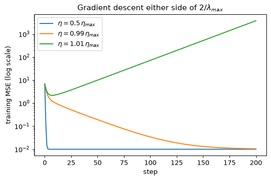
For f up to 0.9 the final MSE is the noise floor, 0.0100 (the noise variance \sigma^2, less the small fraction the fit absorbs), and the distance to the optimum is at rounding error. The f = 0.99 run is still ringing after 200 steps, at 0.0104 and a distance of 0.020. Just over the boundary the loss grows instead of falling, and by f = 1.5 it is astronomically large. A divergence at 1.01 times a threshold computed from the eigenvalues is the cleanest evidence in this module that the theory describes the machine.
A loss that becomes inf or nan is nearly always a step size above 2/\lambda_{\max}. Before
touching anything else, halve \eta and look at the first ten losses. If they now fall, the cause
was the step.
Step 5: bad units
Now break the problem without changing the model. Copy \mathbf{X}, multiply the first column by 1,000, as if a length were recorded in millimetres rather than metres, and add 100 to the second, as if a temperature near 100 °C were recorded in °C rather than as a deviation from 100 °C. The set of functions the model can represent is exactly the same: the new first weight is 1/1000 of the old, and the intercept absorbs the offset. Only the conditioning changes. The condition number is printed for the two changes alone and together, and gradient descent then runs for 100,000 steps at 0.9\,\eta_{\max}, the best step it can safely take.
Xbad = X.copy()
Xbad[:, 0] *= 1000.0
Xbad[:, 1] += 100.0
Xbad_b = np.hstack([Xbad, np.ones((N, 1))])

def kappa_and_limit(Xm):
    lam_m = np.linalg.eigvalsh((2 / len(Xm)) * Xm.T @ Xm)
    return lam_m[-1] / lam_m[0], 2 / lam_m[-1]

Xscale_only = np.hstack([X * np.array([1000.0, 1.0, 1.0]), np.ones((N, 1))])
Xshift_only = np.hstack([X + np.array([0.0, 100.0, 0.0]), np.ones((N, 1))])
print(f"kappa, scaling only : {kappa_and_limit(Xscale_only)[0]:.1e}")
print(f"kappa, offset only  : {kappa_and_limit(Xshift_only)[0]:.1e}")
kappa_bad, eta_max_bad = kappa_and_limit(Xbad_b)
print(f"kappa, both         : {kappa_bad:.1e}")
print(f"eta_max, both       : {eta_max_bad:.1e}")

w_bad_lstsq, *_ = np.linalg.lstsq(Xbad_b, y, rcond=None)
mse_bad = lambda w: np.mean((Xbad_b @ w - y) ** 2)
path_bad = gradient_descent(Xbad_b, y, eta=0.9 * eta_max_bad, steps=100_000)
print(f"lstsq MSE on the bad data : {mse_bad(w_bad_lstsq):.4f}")
print(f"GD MSE after 100,000 steps: {mse_bad(path_bad[-1]):.4f}")
kappa, scaling only : 1.1e+06
kappa, offset only  : 1.0e+08
kappa, both         : 1.0e+10
eta_max, both       : 9.7e-07
lstsq MSE on the bad data : 0.0100
GD MSE after 100,000 steps: 4.2760
A condition number of 10^{10} is not exotic: it is what unscaled engineering data produce. The
step is limited by the largest curvature, which belongs to the column in millimetres, while the
other directions have curvatures many orders of magnitude smaller and barely move in 100,000
steps. After 100,000 steps the training MSE is 4.28, against 0.0100 for lstsq on the same data: the
model is fine and the optimiser has not learned it. lstsq is unaffected, because an
SVD does not care about units to within rounding. The closed form never noticed the problem;
gradient descent, the method that scales to everything else in this series, did. That is why
Section 3 puts standardisation before optimisation.
Step 6: standardise, and map the weights back
Standardising subtracts each column’s training mean and divides by its training standard
deviation, giving columns with mean 0 and variance 1. The offset disappears from the conditioning
(centred columns are orthogonal to the column of ones) and so does the scale. The weights fitted in
the standardised coordinates are mapped back to the original units by w_j = \tilde w_j/s_j and
b = \tilde b - \sum_j \mu_j\tilde w_j/s_j, which follow from substituting
\tilde x_j = (x_j - \mu_j)/s_j into the model. The mapped-back weights must equal lstsq on the
badly scaled problem: standardisation changes the path, not the answer.
mu = Xbad.mean(axis=0)
s = Xbad.std(axis=0)
Z = (Xbad - mu) / s
Zb = np.hstack([Z, np.ones((N, 1))])

kappa_z, _ = kappa_and_limit(Zb)
lam_z = np.linalg.eigvalsh((2 / N) * Zb.T @ Zb)
eta_star_z = 2 / (lam_z[-1] + lam_z[0])
print(f"kappa after standardising = {kappa_z:.2f}")

w_z_star, *_ = np.linalg.lstsq(Zb, y, rcond=None)
print("steps to 1e-6 at eta*     :", steps_to_tolerance(Zb, y, eta_star_z, w_z_star))

w_z = gradient_descent(Zb, y, eta=eta_star_z, steps=50)[-1]
w_orig = np.append(w_z[:3] / s, w_z[3] - np.sum(mu * w_z[:3] / s))
show = lambda v: np.array2string(v, precision=5, suppress_small=True)
print("GD weights, original units:", show(w_orig))
print("lstsq on the bad data     :", show(w_bad_lstsq))
print(f"largest difference        : {np.max(np.abs(w_orig - w_bad_lstsq)):.1e}")
kappa after standardising = 1.22
steps to 1e-6 at eta*     : 6
GD weights, original units: [  0.00149  -2.00962   0.5053  201.65791]
lstsq on the bad data     : [  0.00149  -2.00962   0.5053  201.65791]
largest difference        : 7.1e-13
The condition number returns to about 1, convergence takes a handful of steps, and the mapped-back weights agree with the SVD solution. The first weight, in original units, is about 1.5\times10^{-3}: the true 1.5 divided by the factor of 1,000. The intercept is about 201.7, which is 0.696 + 2.0096\times100: it has absorbed the offset added to the second column. The repair was a change of variables, not a cleverer algorithm. Keep the training mean and standard deviation: any new input must be transformed with these numbers, and Lab 4 shows what happens when it is not.
Step 7: stochastic gradient descent and its noise floor
Section 4 predicts that constant-step SGD does not converge but hovers at a floor, the excess training loss \mathcal{L}(\mathbf{w}_t) - \mathcal{L}(\mathbf{w}^\ast), which for least squares is
with \sigma^2 the residual variance (the code’s s2), as derived in the worked example of that section. The code runs
seven configurations on the original, well-scaled data, each for 50 epochs. Each epoch draws a fresh
permutation (from a generator seeded with 1, separate from the one that made the data), cuts it
into mini-batches of B, and takes one step per batch. After every update it records the excess
loss, using the identity \mathcal{L}(\mathbf{w}) - \mathcal{L}(\mathbf{w}^\ast) = \frac{1}{2}
(\mathbf{w} - \mathbf{w}^\ast)^\top\mathbf{H}(\mathbf{w} - \mathbf{w}^\ast), exact for a
quadratic. The last configuration decays the step as \eta_t = 0.1/(1 + t/200), with t the
update count. The measured floor is the mean excess over the second half of the updates, when the
transient has gone.
def sgd(B, eta, epochs=50, decay_tau=None, seed=1):
    """Mini-batch SGD with per-epoch shuffling; returns the excess loss after every update."""
    gen = np.random.default_rng(seed)
    w = np.zeros(4)
    excess, t = [], 0
    for _ in range(epochs):
        perm = gen.permutation(N)
        for start in range(0, N, B):
            idx = perm[start:start + B]
            grad = (2 / len(idx)) * Xb[idx].T @ (Xb[idx] @ w - y[idx])
            step = eta if decay_tau is None else eta / (1 + t / decay_tau)
            w = w - step * grad
            d = w - w_lstsq
            excess.append(0.5 * d @ H @ d)
            t += 1
    return np.array(excess)

def predicted_floor(B, eta, s2=0.0100):
    return np.sum(eta * s2 * lam / (B * (2 - eta * lam)))

configs = [(200, 0.1, None), (32, 0.1, None), (10, 0.1, None),
           (1, 0.1, None), (1, 0.03, None), (1, 0.01, None), (1, 0.1, 200)]
curves = {}
print(f"{'B':>4} {'eta':>6} {'measured':>10} {'predicted':>10}")
for B, eta, tau in configs:
    ex = sgd(B, eta, decay_tau=tau)
    curves[(B, eta, tau)] = ex
    measured = ex[len(ex) // 2:].mean()
    label = f"{eta}" if tau is None else "decay"
    pred = predicted_floor(B, eta) if tau is None else float("nan")
    print(f"{B:4d} {label:>6} {measured:10.1e} {pred:10.1e}")
print(f"decaying step, last update: {curves[(1, 0.1, 200)][-1]:.1e}")
   B    eta   measured  predicted
 200    0.1    1.7e-05    2.2e-05
  32    0.1    1.0e-04    1.4e-04
  10    0.1    3.1e-04    4.4e-04
   1    0.1    9.6e-03    4.4e-03
   1   0.03    1.3e-03    1.2e-03
   1   0.01    2.7e-04    4.0e-04
   1  decay    3.0e-05        nan
decaying step, last update: 3.1e-06
Read the table down the columns. The measured floor scales as \eta/B: cutting the batch size from 32 to 10 raises it by roughly the factor 3.2, and cutting \eta at B = 1 lowers it in step. The prediction is within a factor of about two for every constant-step row with B < N, which is as good as an additive-noise model deserves. It runs high for the small steps (4.4 against 3.1 at B = 10, in units of 10^{-4}) and low at B = 1, \eta = 0.1 (4.4 against 9.6, in units of 10^{-3}), where the neglected noise that grows with the distance from the optimum is largest. The full-batch row is not a floor: with B = N there is no sampling noise, the run is plain gradient descent, and the number is the mean of a transient that is still shrinking geometrically. The formula does not apply to it, and its closeness to the printed prediction is a coincidence. The decaying step ends at 3\times10^{-6} after the last update, far below every constant-step floor.
Step 8: the plot
The plot puts four runs on log-log axes: full batch, B = 32, B = 1 and B = 1 with decay, each against its own update count. The predicted floors of the two constant-step runs are dashed. Full-batch gradient descent makes one update per epoch, so it has only 50 points; its straight descent is the geometric convergence of Section 3. This is Figure 1.3.
fig, ax = plt.subplots(figsize=(7, 4.5))
spec = [((200, 0.1, None), "full batch, $\\eta = 0.1$", "C0"),
        ((32, 0.1, None), "$B = 32$, $\\eta = 0.1$", "C1"),
        ((1, 0.1, None), "$B = 1$, $\\eta = 0.1$", "C3"),
        ((1, 0.1, 200), "$B = 1$, $\\eta_t = 0.1/(1 + t/200)$", "C2")]
for key, label, colour in spec:
    ex = curves[key]
    ax.loglog(np.arange(1, len(ex) + 1), np.maximum(ex, 1e-12), color=colour,
              lw=1.0, alpha=0.9, label=label)
for (B, eta), colour in [((32, 0.1), "C1"), ((1, 0.1), "C3")]:
    ax.axhline(predicted_floor(B, eta), color=colour, ls="--", lw=1)
ax.set_xlabel("update number")
ax.set_ylabel("excess training loss  $L(w_t) - L(w^*)$")
ax.set_title("SGD hovers at a floor set by $\\eta/B$; decay goes below it")
ax.legend(loc="lower left", fontsize=8)
plt.show()
The B = 32 curve falls quickly, then goes flat near 10^{-4}. The B = 1 curve is flat near 10^{-2} and jagged. The decaying run follows the noisy one at first, then keeps descending after the others have levelled off.
What you should see
- The normal equations,
lstsqand gradient descent agree to three decimals. The residual RMS equals the noise standard deviation: no recoverable signal is left unexplained. - The divergence boundary is sharp and where the eigenvalue analysis puts it: 0.99\,\eta_{\max} converges (slowly, ringing), 1.01\,\eta_{\max} explodes.
- With bad units gradient descent appears not to learn although the model is fine. Standardising
restores convergence in a handful of steps, and the weights mapped back to the original units
equal the
lstsqsolution. The fix is a change of variables, not a new algorithm. The closed form never noticed the problem. - Constant-step SGD hovers at a floor roughly proportional to \eta/B. The predictions agree within about a factor of two. A decaying step goes below every floor.
Try this
- Add a fifth column equal to 0.99\times column 0 plus 0.01\times noise, standardise everything and watch \kappa and the gradient descent step count grow. This is conditioning from correlation, which no rescaling removes.
- Replace the fixed step by backtracking: halve \eta until the loss decreases, and compare the number of steps with those at \eta^\ast.
- Time
np.linalg.lstsqagainst 100 gradient descent steps for N = 10^6, d = 100, and decide which you would use. Then decide which you would use for d = 10^5. - Run SGD with indices drawn independently with replacement instead of shuffled epochs, and compare the floors with the table: the worked example in Section 4 says what to expect.
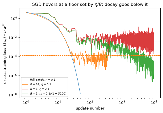
Lab 2 — Logistic regression from scratch, and the metrics a decision needs
Goal. You implement regularised logistic regression with a numerically stable loss and a gradient you have checked, train it by gradient descent, and confirm that it matches scikit-learn once both have converged. You then measure the classifier the way a decision needs: a confusion matrix, the threshold that meets a recall target, the ROC and precision–recall curves, and calibration, including a constant predictor that is better calibrated than the model and useless. You finish by removing the penalty on separable data and watching the weights grow without bound. The data ship with scikit-learn, so there is no download, and the lab runs in a few seconds.
Step 1: the data
scikit-learn’s breast-cancer data have 569 cases and 30 numeric features computed from images of
cell nuclei. The library codes malignant as 0, which makes accuracy and recall easy to misread. The
question an engineer asks is “is this a defect?”, so the defect, here malignant, must be the
positive class: flip the target with y = 1 - target. The split is stratified, so that the
training and test sets keep the class proportions, and the standardisation uses training statistics
only. Test data must never contribute to anything that is fitted, and that includes the mean and
the standard deviation.
import numpy as np
import matplotlib.pyplot as plt
from scipy.special import expit
from sklearn.datasets import load_breast_cancer
from sklearn.model_selection import train_test_split
from sklearn.linear_model import LogisticRegression
from sklearn.metrics import (confusion_matrix, roc_auc_score, average_precision_score,
                             roc_curve, precision_recall_curve, brier_score_loss)

np.set_printoptions(precision=4, suppress=True)
np.random.seed(0)

data = load_breast_cancer()
y_all = 1 - data.target                      # malignant = 1 (scikit-learn codes it as 0)
print("malignant:", int(y_all.sum()), " benign:", int((1 - y_all).sum()))

X_tr, X_te, y_tr, y_te = train_test_split(
    data.data, y_all, test_size=0.25, stratify=y_all, random_state=0)
print("train:", X_tr.shape, int(y_tr.sum()), "malignant")
print("test: ", X_te.shape, int(y_te.sum()), "malignant")

mu, sd = X_tr.mean(axis=0), X_tr.std(axis=0)
A_tr = np.hstack([(X_tr - mu) / sd, np.ones((len(X_tr), 1))])   # last column: intercept
A_te = np.hstack([(X_te - mu) / sd, np.ones((len(X_te), 1))])
N = len(y_tr)
malignant: 212  benign: 357
train: (426, 30) 159 malignant
test:  (143, 30) 53 malignant
Step 2: the loss, its gradient and the step-size bound
With logit z = \mathbf{a}^\top\mathbf{w} and probability \hat p = \sigma(z), the per-example
negative log-likelihood is \ln(1 + e^{z}) - yz, derived in Section 6. Computed naively,
e^{z} overflows for large z; np.logaddexp(0, z) evaluates \ln(e^0 + e^z) without forming
the exponential. The mean loss adds the penalty \lambda\lVert\mathbf{w}\rVert^2 on the 30 feature
weights, not on the intercept, with \lambda = 1/(2NC) so that it matches scikit-learn’s
C = 1. The gradient is \frac{1}{N}\mathbf{A}^\top(\hat{\mathbf{p}} - \mathbf{y}) + 2\lambda
\mathbf{w} with the penalty term zero for the intercept.
The Hessian of the data term is \frac{1}{N}\mathbf{A}^\top\mathrm{diag}(\hat p(1 - \hat p)) \mathbf{A}, and \hat p(1 - \hat p) \le \frac{1}{4}, so its largest eigenvalue is at most L = \lambda_{\max}(\mathbf{A}^\top\mathbf{A}/N)/4. Gradient descent with \eta < 2/L is then safe. Print the bound.
C = 1.0
lam_reg = 1.0 / (2 * N * C)                  # ridge strength matching scikit-learn's C
mask = np.r_[np.ones(30), 0.0]               # the intercept is not penalised

def loss_fn(w, A=A_tr, y=y_tr, lam=lam_reg):
    z = A @ w
    return np.mean(np.logaddexp(0, z) - y * z) + lam * np.sum((mask * w) ** 2)

def grad_fn(w, A=A_tr, y=y_tr, lam=lam_reg):
    p = expit(A @ w)
    return A.T @ (p - y) / len(y) + 2 * lam * mask * w

L = np.linalg.eigvalsh(A_tr.T @ A_tr / N)[-1] / 4
print(f"curvature bound L = {L:.2f}; GD is safe for eta < 2/L = {2 / L:.2f}")
curvature bound L = 3.39; GD is safe for eta < 2/L = 0.59
The step \eta = 0.5 is used below. The bound is for a loss that curves as sharply as it ever can; near the minimum it curves much less, which is why the bound is sufficient but not necessary for this non-quadratic loss, as Section 6 notes.
Step 3: check the gradient
A hand-written gradient is the most likely place for a silent bug, and a wrong gradient does not crash: it makes training slow or wrong. The check compares it with central differences, (\mathcal{L}(\mathbf{w} + \epsilon\mathbf{e}_j) - \mathcal{L}(\mathbf{w} - \epsilon\mathbf{e}_j))/2\epsilon, at a random point, using the relative error \lVert g_{\text{num}} - g\rVert / \lVert g_{\text{num}} + g\rVert. A correct gradient gives an error far below 10^{-6}. Module 02 makes this check a routine part of writing backpropagation.
gen = np.random.default_rng(0)
w_probe = 0.1 * gen.normal(size=31)
g = grad_fn(w_probe)
eps = 1e-6
g_num = np.array([(loss_fn(w_probe + eps * e) - loss_fn(w_probe - eps * e)) / (2 * eps)
                  for e in np.eye(31)])
rel = np.linalg.norm(g_num - g) / np.linalg.norm(g_num + g)
print(f"relative error of the gradient: {rel:.1e}")
relative error of the gradient: 1.2e-10
Step 4: train by gradient descent
Run 20,000 steps of full-batch gradient descent from zero at \eta = 0.5 and print the loss at steps 10, 100, 1,000 and 20,000. The fast fall at first and the long tail after it are typical of a problem whose curvature differs by directions: the standardised features of this data are strongly correlated (the 30 measurements are largely different ways of describing size).
w = np.zeros(31)
eta = 0.5
history = {}
for step in range(1, 20_001):
    w = w - eta * grad_fn(w)
    if step in (10, 100, 1_000, 20_000):
        history[step] = loss_fn(w)
for step, value in history.items():
    print(f"step {step:6d}: loss {value:.4f}")
w_gd = w.copy()
print(f"gradient norm at the end: {np.linalg.norm(grad_fn(w_gd)):.1e}")
step     10: loss 0.1233
step    100: loss 0.0760
step   1000: loss 0.0685
step  20000: loss 0.0684
gradient norm at the end: 2.3e-14
Step 5: compare with scikit-learn
LogisticRegression(C=1.0) minimises the same objective: \sum_i (negative log-likelihood) +
\frac{1}{2C}\lVert\mathbf{w}\rVert^2, which is N times ours with \lambda = 1/(2NC). The default
convergence tolerance, tol=1e-4, stops the solver early, and the coefficients then differ from
the true minimum by an amount that is easy to mistake for a bug in one implementation or the
other. The code fits with a tight tolerance and with the default and prints the largest coefficient
difference from the gradient descent solution in each case.
def fit_sklearn(tol):
    m = LogisticRegression(C=1.0, tol=tol, max_iter=10_000)
    m.fit(A_tr[:, :30], y_tr)
    return np.append(m.coef_.ravel(), m.intercept_[0])

w_tight = fit_sklearn(1e-8)
w_default = fit_sklearn(1e-4)
print(f"tol = 1e-8: largest coefficient difference = {np.max(np.abs(w_tight - w_gd)):.1e}")
print(f"tol = 1e-4: largest coefficient difference = {np.max(np.abs(w_default - w_gd)):.1e}")
tol = 1e-8: largest coefficient difference = 9.4e-07
tol = 1e-4: largest coefficient difference = 1.6e-02
With a tight tolerance the two solutions agree to about 10^{-6}. With the default, they differ in the second decimal. The model is the same; the stopping rule is not. This is worth knowing before blaming either implementation for a small disagreement.
Step 6: the confusion matrix on the test set
Probabilities become decisions at a threshold, here 0.5. The confusion matrix counts the four outcomes; rows are the true class and columns the prediction, with negative (benign) first. Accuracy is only meaningful next to the baseline of always predicting the majority class, whose accuracy is the proportion of the majority class in the test set.
p_te = expit(A_te @ w_gd)
pred = (p_te >= 0.5).astype(int)
tn, fp, fn, tp = confusion_matrix(y_te, pred).ravel()
print("confusion matrix [[TN, FP], [FN, TP]]:")
print(np.array([[tn, fp], [fn, tp]]))

accuracy = (tp + tn) / len(y_te)
precision = tp / (tp + fp)
recall = tp / (tp + fn)
f1 = 2 * precision * recall / (precision + recall)
baseline = 1 - y_te.mean()
print(f"accuracy {accuracy:.3f}  precision {precision:.3f}  recall {recall:.3f}  "
      f"F1 {f1:.3f}")
print(f"majority-class baseline accuracy {baseline:.3f}")
confusion matrix [[TN, FP], [FN, TP]]:
[[90  0]
 [ 2 51]]
accuracy 0.986  precision 1.000  recall 0.962  F1 0.981
majority-class baseline accuracy 0.629
Accuracy near 0.99 sounds excellent, and it means something only next to a baseline of 0.629 that needs no model. The errors are not symmetric in cost: a false negative here is a malignant case called benign. Precision answers “of those flagged, how many are real?” and recall answers “of the real ones, how many were flagged?”. Neither is visible in accuracy.
Step 7: ROC and precision–recall curves
The curves sweep the threshold instead of fixing it. The ROC curve plots recall (true-positive rate) against the false-positive rate; its area, the AUC, is the probability that a random positive scores above a random negative. The precision–recall curve plots precision against recall; a model that ranks at random has precision equal to the prevalence, 53/143 = 0.371, so that is its baseline, not 0.5. The marked point is the threshold-0.5 decision of the last step.
auc = roc_auc_score(y_te, p_te)
ap = average_precision_score(y_te, p_te)
print(f"ROC AUC           = {auc:.3f}")
print(f"average precision = {ap:.3f}")

fpr, tpr, _ = roc_curve(y_te, p_te)
prec_c, rec_c, thr_c = precision_recall_curve(y_te, p_te)

fig, axes = plt.subplots(1, 2, figsize=(10, 4.2))
axes[0].plot(fpr, tpr, label=f"logistic regression (AUC {auc:.3f})")
axes[0].plot([0, 1], [0, 1], "k--", lw=1, label="chance")
axes[0].plot(fp / (fp + tn), recall, "o", color="C3", label="threshold 0.5")
axes[0].set_xlabel("false-positive rate")
axes[0].set_ylabel("recall (true-positive rate)")
axes[0].set_title("ROC curve, 143 test cases")
axes[0].legend(loc="lower right")
axes[1].plot(rec_c, prec_c, label=f"logistic regression (AP {ap:.3f})")
axes[1].axhline(y_te.mean(), color="k", ls="--", lw=1, label="chance (prevalence 0.371)")
axes[1].plot(recall, precision, "o", color="C3", label="threshold 0.5")
axes[1].set_xlabel("recall")
axes[1].set_ylabel("precision")
axes[1].set_ylim(0.3, 1.05)
axes[1].set_title("Precision-recall curve, 143 test cases")
axes[1].legend(loc="lower left")
plt.tight_layout()
plt.show()
ROC AUC           = 0.996
average precision = 0.994
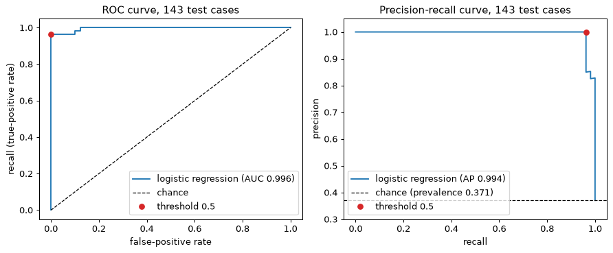
The ROC curve hugs the top-left corner: the ranking is excellent. An AUC says nothing, however, about where to put the threshold, and that is the decision.
Step 8: a threshold for a recall target
Suppose a missed malignant case is unacceptable and the requirement is a recall of at least 0.98.
precision_recall_curve returns precision and recall at every threshold at which the
predictions change. Scanning from the highest threshold down gives the largest threshold that
meets the target, which is the one with the best precision among those that do.
def threshold_for_recall(target):
    ok = np.where(rec_c[:-1] >= target)[0]           # rec_c is non-increasing in the index
    i = ok[-1]
    return thr_c[i], prec_c[i], rec_c[i]

print(f"{'target recall':>14} {'threshold':>10} {'precision':>10} {'recall':>8}")
for target in [0.95, 0.98, 1.0]:
    thr, pr, rc = threshold_for_recall(target)
    print(f"{target:14.2f} {thr:10.3f} {pr:10.3f} {rc:8.3f}")
 target recall  threshold  precision   recall
          0.95      0.509      1.000    0.962
          0.98      0.218      0.852    0.981
          1.00      0.116      0.828    1.000
The ranking is excellent, and the threshold is still a decision. Meeting a recall of 0.98 needs a threshold of 0.218 and costs precision 0.852; catching every one of the 53 malignant cases needs 0.116 and a precision of 0.828, roughly one flagged case in six benign. Whether that is acceptable depends on what a false alarm costs against a miss, which is a question about the application, not about the model. Note also that these are test-set numbers from 53 positives: the thresholds themselves would move with another sample. The threshold should be chosen on validation data and only reported on test data; here the test set is used for illustration, and Lab 4 shows the right protocol.
Step 9: calibration
A model is calibrated if, among cases given probability 0.8, about 80% are positive. The reliability diagram groups the test cases into 5 equal-width bins of predicted probability and plots the fraction of positives in each against the bin’s mean prediction. The expected calibration error (ECE) is the weighted mean gap, \sum_b \frac{n_b}{n}\lvert\text{freq}_b - \text{conf}_b\rvert over the n test cases, as defined in Section 7, and the Brier score is the mean squared error of the probabilities, \frac{1}{n}\sum_i(\hat p_i - y_i)^2. Both are computed, and the diagram is this lab’s version of Figure 1.6 in Section 7. Then score the constant predictor that outputs the training prevalence, 159/426 = 0.373, for every case.
def binned_calibration(p, y, n_bins=5):
    edges = np.linspace(0, 1, n_bins + 1)
    idx = np.clip(np.digitize(p, edges[1:-1]), 0, n_bins - 1)
    rows, ece = [], 0.0
    for b in range(n_bins):
        sel = idx == b
        if sel.any():
            rows.append((p[sel].mean(), y[sel].mean(), sel.sum()))
            ece += sel.mean() * abs(y[sel].mean() - p[sel].mean())
    return np.array(rows), ece

rows, ece = binned_calibration(p_te, y_te)
brier = brier_score_loss(y_te, p_te)
print(f"model:    Brier {brier:.3f}  ECE {ece:.3f}  AUC {auc:.3f}")
for mean_p, frac, n in rows:
    print(f"   bin: mean prediction {mean_p:.3f}, fraction positive {frac:.3f}, n = {int(n)}")

p_const = np.full(len(y_te), y_tr.mean())
_, ece_c = binned_calibration(p_const, y_te)
print(f"constant: Brier {brier_score_loss(y_te, p_const):.3f}  ECE {ece_c:.3f}  "
      f"AUC {roc_auc_score(y_te, p_const):.3f}")

fig, ax = plt.subplots(figsize=(5, 4.5))
ax.plot([0, 1], [0, 1], "k--", lw=1, label="perfect calibration")
ax.plot(rows[:, 0], rows[:, 1], "o-", label="logistic regression")
for mean_p, frac, n in rows:
    ax.annotate(f"n={int(n)}", (mean_p, frac), textcoords="offset points", xytext=(5, -12),
                fontsize=8)
ax.set_xlabel("mean predicted probability in the bin")
ax.set_ylabel("fraction of positives in the bin")
ax.set_title("Reliability diagram, 5 bins, 143 test cases")
ax.legend(loc="upper left")
plt.show()
model:    Brier 0.023  ECE 0.023  AUC 0.996
   bin: mean prediction 0.015, fraction positive 0.012, n = 82
   bin: mean prediction 0.278, fraction positive 0.143, n = 7
   bin: mean prediction 0.473, fraction positive 0.250, n = 4
   bin: mean prediction 0.665, fraction positive 1.000, n = 3
   bin: mean prediction 0.996, fraction positive 1.000, n = 47
constant: Brier 0.233  ECE 0.003  AUC 0.500
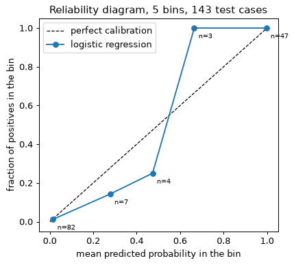
The model’s ECE is small, but 143 cases spread over 5 bins leave only a handful of cases in the middle bins, so each bin’s fraction positive is a noisy estimate and ECE is biased upward by that noise (Section 7). The constant predictor shows why ECE cannot be used alone. Its ECE is smaller than the model’s, because the overall frequency of positives in the test set is close to the training prevalence, so its single bin is nearly calibrated. Yet its Brier score is ten times worse and its AUC is exactly 0.5: it says nothing about any individual case. Calibration is not discrimination, and a metric of one kind cannot stand in for the other.
Step 10: what happens without a penalty on separable data
If a hyperplane separates the classes perfectly, the likelihood keeps increasing as the weights grow along the separating direction, because every example’s logit moves further from zero on the correct side. Without a penalty there is no minimum: \lVert\mathbf{w}\rVert grows for ever, and the loss falls towards zero. The penalty is what makes the minimum exist (Section 6). With 30 features and 426 training cases the training set of this lab is separable, which the run confirms by driving the training errors to zero with \lambda = 0. The step is \eta = 1.0, above the bound for the penalised problem, which is acceptable here because the Hessian shrinks as the probabilities saturate.
w_sep = np.zeros(31)
checkpoints = {100, 1_000, 10_000, 100_000}
for step in range(1, 100_001):
    w_sep = w_sep - 1.0 * grad_fn(w_sep, lam=0.0)
    if step in checkpoints:
        print(f"step {step:7d}: ||w|| = {np.linalg.norm(w_sep):6.1f}   "
              f"loss = {loss_fn(w_sep, lam=0.0):.4f}")
train_errors = int(np.sum((A_tr @ w_sep >= 0).astype(int) != y_tr))
print("training errors:", train_errors)
step     100: ||w|| =    3.2   loss = 0.0584
step    1000: ||w|| =    6.2   loss = 0.0413
step   10000: ||w|| =   16.1   loss = 0.0256
step  100000: ||w|| =   51.2   loss = 0.0088
training errors: 0
The norm keeps rising and never settles: 3.2, 6.2, 16.1 and 51.2 at 100, 1,000, 10,000 and 100,000 steps, while the loss falls from 0.058 to 0.0088 and the training errors reach zero. For exactly separable data the growth is eventually only logarithmic in the step count, but this run has not reached that regime (each tenfold increase in steps multiplies the norm by 1.9, then 2.6, then 3.2), so do not extrapolate from it. What matters is that there is no limit: the unpenalised “solution” does not exist, and what you get is whatever the run had reached when you stopped it. This is why scikit-learn defaults to an L2 penalty, and why a coefficient of 10^{3} in an unpenalised logistic regression is a warning, not a finding.
What you should see
- The from-scratch model and scikit-learn agree once both have converged. A disagreement of 10^{-2} comes from a solver tolerance, not from the model.
- AUC near 0.996 says the ranking is excellent, but the threshold is still a decision: catching every malignant case costs precision of about 0.83 instead of 1.00.
- Accuracy of 0.986 means something only next to the 0.629 baseline.
- Without a penalty on separable data \lVert\mathbf{w}\rVert grows without limit (3.2 to 51 over three decades of steps) and the probabilities saturate. The L2 penalty is what prevents it.
- ECE alone would rank the constant predictor above the model; the Brier score and the AUC do not. Calibration is not discrimination.
Try this
- Implement softmax regression on
load_iriswith your own gradient, (\hat{\mathbf{P}} - \mathbf{Y})^\top\mathbf{X}/N, and compare withLogisticRegression. - Repeat step 4 with \eta = 2 and \eta = 5. The loss still falls: the bound \eta < 2/L is sufficient, not necessary, for this non-quadratic loss.
- Recalibrate with
CalibratedClassifierCV(method='sigmoid', cv=5)on the training set and compare Brier scores and the reliability diagram. - Rerun the threshold search of step 8 on the training set with cross-validated probabilities, fix the threshold, then report precision and recall on the test set. How far do they move?
Lab 3 — Polynomials: capacity, bias–variance and the ridge path
Goal. You reproduce the capacity curve of Section 8 on twenty noisy points of \sin(2\pi x), estimate the bias² and variance of each polynomial degree by Monte Carlo and check them against the exact formulas for a fixed design, trace the ridge path at degree 15, and choose the penalty by five-fold cross-validation. The lab then repeats the experiment with ten times as much data. Synthetic data, NumPy only, no download; it runs in a few seconds.
Step 1: the data, and why the basis matters
The true function is f(x) = \sin(2\pi x) and the noise has standard deviation \sigma = 0.3. The training inputs are a fixed design, 20 evenly spaced points on [0, 1], and only the noise is random. A fixed design keeps the experiment clean: random inputs leave gaps near the ends, and a high-degree polynomial then has a variance so large there that it swamps every plot. The validation and test inputs are drawn uniformly, 1,000 and 10,000 of them, and the draws happen in a fixed order from one generator, so the numbers are reproducible.
The features are Legendre polynomials P_0(t), \dots, P_d(t) in t = 2x - 1, which maps [0, 1] onto [-1, 1]. They span exactly the same functions as the monomials x^k, so the fitted curve is the same in exact arithmetic; what changes is the conditioning of the design matrix. The condition number of the degree-15 design is printed for both bases.
import numpy as np
import matplotlib.pyplot as plt
from numpy.polynomial import legendre as L

np.set_printoptions(precision=3, suppress=True)
np.random.seed(0)
SIGMA = 0.3
f = lambda x: np.sin(2 * np.pi * x)

def make_data(n_train, seed=0):
    gen = np.random.default_rng(seed)
    x_tr = np.linspace(0, 1, n_train)                       # fixed design
    y_tr = f(x_tr) + SIGMA * gen.normal(size=n_train)
    x_va = gen.uniform(0, 1, 1000)
    y_va = f(x_va) + SIGMA * gen.normal(size=1000)
    x_te = gen.uniform(0, 1, 10_000)
    y_te = f(x_te) + SIGMA * gen.normal(size=10_000)
    return x_tr, y_tr, x_va, y_va, x_te, y_te

x_tr, y_tr, x_va, y_va, x_te, y_te = make_data(20)
phi = lambda x, d: L.legvander(2 * x - 1, d)                # shape (len(x), d + 1)

t = 2 * x_tr - 1
print(f"condition number, Legendre design, d = 15: {np.linalg.cond(phi(x_tr, 15)):.1f}")
print(f"condition number, monomial design, d = 15: "
      f"{np.linalg.cond(np.vander(t, 16, increasing=True)):.1e}")
condition number, Legendre design, d = 15: 46.7
condition number, monomial design, d = 15: 6.7e+05
The Legendre basis is nearly orthogonal on the interval, which keeps the condition number small. The monomial basis has columns that are all close to one another for large powers, and its condition number is four orders of magnitude worse. The normal equations square the condition number, so with monomials at degree 15 they lose most of the digits of double precision. We use Legendre throughout.
Step 2: the capacity curve
Fit degrees 0 to 15 by least squares (np.linalg.lstsq) and record the root mean squared error on
the training and validation sets. The training error cannot increase with the degree, because each
model contains the previous one. The validation error is the estimate of how the fit will do on new
data: it should fall to a minimum and then rise.
def rmse(a, b):
    return float(np.sqrt(np.mean((a - b) ** 2)))

def fit_ls(x, y, d):
    w, *_ = np.linalg.lstsq(phi(x, d), y, rcond=None)
    return w

degrees = list(range(16))
train_err, val_err = [], []
for d in degrees:
    w = fit_ls(x_tr, y_tr, d)
    train_err.append(rmse(phi(x_tr, d) @ w, y_tr))
    val_err.append(rmse(phi(x_va, d) @ w, y_va))

print(" degree  train RMSE  validation RMSE")
for d in degrees:
    print(f"{d:7d} {train_err[d]:11.3f} {val_err[d]:16.3f}")
print("best validation degree:", int(np.argmin(val_err)))
 degree  train RMSE  validation RMSE
      0       0.850            0.769
      1       0.655            0.536
      2       0.648            0.540
      3       0.217            0.354
      4       0.217            0.354
      5       0.183            0.360
      6       0.181            0.360
      7       0.178            0.361
      8       0.173            0.364
      9       0.173            0.365
     10       0.163            0.367
     11       0.141            0.393
     12       0.141            0.393
     13       0.128            0.385
     14       0.123            0.434
     15       0.112            0.720
best validation degree: 4
The training RMSE falls with every degree and reaches 0.11 at degree 15, far below the noise level of 0.3: the fit is following the noise. The validation RMSE falls to about 0.35 at degrees 3 and 4 and climbs to about 0.72 at degree 15. Degrees 3 and 4 are nearly identical because \sin(2\pi x) is odd about x = \tfrac12: the even Legendre term added at degree 4 has a true coefficient of exactly zero on this symmetric design, so it can only fit noise.
Step 3: the fits themselves
The left panel draws the true function, the data and the fits of degrees 1, 3 and 15 on a fine grid; the right panel draws the RMSE curves. Degree 1 is a straight line through a sine wave (underfit), degree 3 follows it, and degree 15 passes close to every training point and oscillates between them, with the largest swings near the ends, where 20 points constrain the polynomial least. This is Figure 1.7.
grid = np.linspace(0, 1, 201)
fig, axes = plt.subplots(1, 2, figsize=(11, 4.3))
axes[0].plot(grid, f(grid), "k", lw=1.5, label=r"true $\sin(2\pi x)$")
axes[0].plot(x_tr, y_tr, "o", color="grey", ms=4, label="20 training points")
for d, colour in [(1, "C0"), (3, "C2"), (15, "C3")]:
    axes[0].plot(grid, phi(grid, d) @ fit_ls(x_tr, y_tr, d), color=colour, label=f"degree {d}")
axes[0].set_ylim(-2.2, 2.2)
axes[0].set_xlabel("x")
axes[0].set_ylabel("y")
axes[0].set_title("Least-squares polynomial fits to 20 noisy points")
axes[0].legend(fontsize=8)

axes[1].plot(degrees, train_err, "o-", label="training")
axes[1].plot(degrees, val_err, "s-", label="validation (1,000 points)")
axes[1].axhline(SIGMA, color="k", ls="--", lw=1, label="noise level $\\sigma$ = 0.3")
axes[1].set_xlabel("polynomial degree")
axes[1].set_ylabel("RMSE")
axes[1].set_title("Training error falls; validation error turns up")
axes[1].legend(fontsize=8)
plt.tight_layout()
plt.show()
Step 4: bias² and variance, by simulation and exactly
For a fixed design, the expected squared error at a point x splits, as in Section 8, into bias² + variance + \sigma^2, where bias is the gap between the average prediction (over training sets) and the truth and variance is the spread of the prediction around its average. Both can be estimated by simulation: draw R = 200 new sets of noise on the same inputs, refit each, and average over a grid of 201 points.
For least squares on a fixed design there is also an exact answer. The fitted values at the grid are linear in the targets, \hat f_{\text{grid}} = \mathbf{S}\mathbf{y}, with the smoother matrix \mathbf{S} = \boldsymbol{\Phi}_g(\boldsymbol{\Phi}^\top\boldsymbol{\Phi})^{-1} \boldsymbol{\Phi}^\top. Using the QR factorisation \boldsymbol{\Phi} = \mathbf{QR} this is \boldsymbol{\Phi}_g\mathbf{R}^{-1}\mathbf{Q}^\top, which avoids forming \boldsymbol{\Phi}^\top\boldsymbol{\Phi}. The mean prediction is \mathbf{S}f(x_{\text{train}}), so the bias² is the mean over the grid of (\mathbf{S}f_{\text{train}} - f_{\text{grid}})^2, and the variance is \sigma^2 times the mean over the grid of the row sums of \mathbf{S}^2.
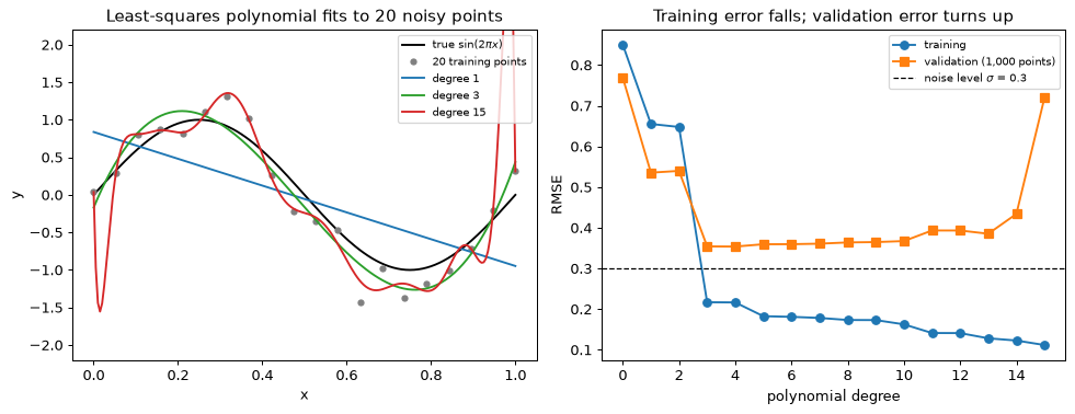
gen_mc = np.random.default_rng(1)
R_DRAWS = 200
noise = SIGMA * gen_mc.normal(size=(R_DRAWS, 20))
Y_sims = f(x_tr)[None, :] + noise                            # (200, 20): fresh targets, same x

def bias_var_mc(d):
    P, Pg = phi(x_tr, d), phi(grid, d)
    W, *_ = np.linalg.lstsq(P, Y_sims.T, rcond=None)         # (d+1, 200): one fit per draw
    preds = Pg @ W                                           # (201, 200)
    return np.mean((preds.mean(axis=1) - f(grid)) ** 2), np.mean(preds.var(axis=1))

def bias_var_exact(d):
    Q, Rm = np.linalg.qr(phi(x_tr, d))
    S = phi(grid, d) @ np.linalg.solve(Rm, Q.T)             # (201, 20) smoother matrix
    return np.mean((S @ f(x_tr) - f(grid)) ** 2), SIGMA**2 * np.mean(np.sum(S**2, axis=1))

print("        Monte Carlo (R = 200)          exact")
print("degree  bias^2  variance  total      bias^2  variance  total")
for d in [0, 1, 2, 3, 4, 5, 9, 12, 15]:
    b_m, v_m = bias_var_mc(d)
    b_e, v_e = bias_var_exact(d)
    print(f"{d:6d} {b_m:7.4f} {v_m:9.4f} {b_m + v_m + SIGMA**2:7.4f}  "
          f"{b_e:9.4f} {v_e:8.4f} {b_e + v_e + SIGMA**2:7.4f}")
        Monte Carlo (R = 200)          exact
degree  bias^2  variance  total      bias^2  variance  total
     0  0.4975    0.0044  0.5919     0.4975   0.0045  0.5920
     1  0.2051    0.0084  0.3034     0.2051   0.0086  0.3037
     2  0.2051    0.0119  0.3070     0.2051   0.0124  0.3075
     3  0.0051    0.0154  0.1104     0.0052   0.0161  0.1113
     4  0.0051    0.0189  0.1140     0.0052   0.0198  0.1150
     5  0.0002    0.0226  0.1128     0.0000   0.0236  0.1136
     9  0.0002    0.0414  0.1316     0.0000   0.0422  0.1322
    12  0.0006    0.0742  0.1648     0.0000   0.0754  0.1654
    15  0.0022    0.9209  1.0130     0.0000   0.8737  0.9637
The two blocks agree to within a few per cent on the variance. The Monte Carlo bias² is larger than the exact value, and the reason is the estimator itself: the average of R = 200 noisy predictions has its own sampling variance, \text{variance}/R, and squaring the average adds that to the bias². At degree 15, with variance 0.87, the expected inflation is 0.87/200 \approx 0.004; this run shows 0.002, which is within the scatter of a quantity whose variance is concentrated near the two ends of the interval, where few of the 201 grid points carry it. The exact bias² there is zero to four decimals, because a degree-15 polynomial can follow \sin(2\pi x) at 20 points almost perfectly. The Monte Carlo total at degree 15 is correspondingly 1.01 against the exact 0.96. The totals, bias² + variance + \sigma^2, are the expected squared error at a new point: at degree 3 about 0.111 (RMSE 0.334, close to the 0.354 that the one validation set gave) and at degree 15 about 0.96 (RMSE 0.98). Bias² falls in pairs (degrees 1 and 2, then 3 and 4) for the oddness reason of step 2.
The variance grows with the degree, slowly at first and then violently at 15, where 16 parameters are fitted by 20 points and the model nearly interpolates. Averaged over the 20 training inputs the variance is exactly \sigma^2(d + 1)/N, which is 0.072 at degree 15; the 0.87 is over a grid that includes the ends, where the polynomial is far from the data.
Step 5: the ridge path at degree 15
Keep the 16 features of degree 15 and shrink them instead of removing them. Ridge regression minimises \frac{1}{N}\lVert\mathbf{y} - \boldsymbol\Phi\mathbf{w}\rVert^2 + \lambda\lVert\mathbf{w}\rVert^2 and has the solution (\boldsymbol\Phi^\top\boldsymbol\Phi + \lambda N\mathbf{I}')\mathbf{w} = \boldsymbol\Phi^\top\mathbf{y}, where \mathbf{I}' is the identity with a zero for the constant term, so that the intercept is not shrunk. The code sweeps \lambda over 23 values from 10^{-10} to 10 and prints the training and validation RMSE and \lVert\mathbf{w}\rVert. The Legendre basis matters here too: with standardised monomials the penalty acts on badly scaled columns, and even \lambda = 10^{-10} would already regularise, so the overfitting end of the path would never appear.
def fit_ridge(x, y, d, lam):
    P = phi(x, d)
    pen = np.eye(P.shape[1])
    pen[0, 0] = 0.0                                          # leave the constant term alone
    return np.linalg.solve(P.T @ P + lam * len(y) * pen, P.T @ y)

lams = np.logspace(-10, 1, 23)
path = []
print("      lambda  train RMSE  val RMSE   ||w||")
for lam in lams:
    w = fit_ridge(x_tr, y_tr, 15, lam)
    row = (lam, rmse(phi(x_tr, 15) @ w, y_tr), rmse(phi(x_va, 15) @ w, y_va),
           np.linalg.norm(w))
    path.append(row)
for i in range(0, 23, 2):
    print(f"{path[i][0]:12.2e} {path[i][1]:11.3f} {path[i][2]:9.3f} {path[i][3]:9.2f}")
best_val = min(path, key=lambda r: r[2])
print(f"best validation RMSE {best_val[2]:.3f} at lambda = {best_val[0]:.3f}")

fig, ax = plt.subplots(figsize=(6.5, 4.2))
ax.semilogx(lams, [r[1] for r in path], "o-", ms=3, label="training")
ax.semilogx(lams, [r[2] for r in path], "s-", ms=3, label="validation")
ax.axhline(SIGMA, color="k", ls="--", lw=1, label="noise level $\\sigma$")
ax.set_xlabel("regularisation strength $\\lambda$")
ax.set_ylabel("RMSE")
ax.set_title("Ridge path at degree 15: from interpolation to underfitting")
ax.legend()
plt.show()
      lambda  train RMSE  val RMSE   ||w||
    1.00e-10       0.112     0.720      2.98
    1.00e-09       0.112     0.720      2.98
    1.00e-08       0.112     0.720      2.98
    1.00e-07       0.112     0.720      2.98
    1.00e-06       0.112     0.719      2.98
    1.00e-05       0.112     0.710      2.95
    1.00e-04       0.112     0.641      2.73
    1.00e-03       0.117     0.441      2.14
    1.00e-02       0.133     0.362      1.85
    1.00e-01       0.319     0.348      1.22
    1.00e+00       0.702     0.629      0.33
    1.00e+01       0.832     0.751      0.07
best validation RMSE 0.335 at lambda = 0.032
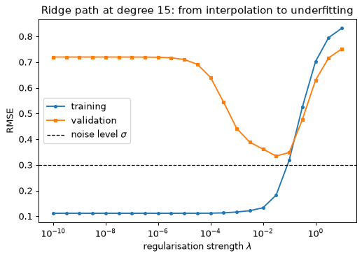
At the left, with almost no penalty, the fit is the unregularised degree-15 fit: training RMSE near 0.11, validation near 0.72. As \lambda grows the weights shrink, the training error rises and the validation error falls; at large \lambda both rise together as the model is flattened towards a constant. It is the same U-shape as in the degree curve, now along a continuous axis that is easier to search. The validation minimum, about 0.335 near \lambda = 0.03, is lower than the best unregularised degree of step 2 (0.354).
Step 6: choosing λ by cross-validation
A validation set of 1,000 points is a luxury. With 20 training points an honest procedure uses only those: five-fold cross-validation, in which the points are permuted, cut into five folds of four, and each fold in turn is predicted by a model fitted to the other 16. The mean of the five fold errors estimates the error at that \lambda; their standard deviation over \sqrt5 is a rough standard error (Section 8). The one-standard-error rule picks the strongest penalty whose mean error is within one standard error of the minimum. After choosing \lambda, refit on all 20 points and evaluate once on the 10,000-point test set, alongside unregularised degrees 3 and 15.
perm = np.random.default_rng(0).permutation(20)
folds = np.array_split(perm, 5)

def cv_scores(lam):
    errs = []
    for k in range(5):
        va = folds[k]
        tr = np.concatenate([folds[j] for j in range(5) if j != k])
        w = fit_ridge(x_tr[tr], y_tr[tr], 15, lam)
        errs.append(np.mean((phi(x_tr[va], 15) @ w - y_tr[va]) ** 2))
    return np.mean(errs), np.std(errs, ddof=1) / np.sqrt(5)

cv = np.array([cv_scores(lam) for lam in lams])
i_min = int(np.argmin(cv[:, 0]))
within = np.where(cv[:, 0] <= cv[i_min, 0] + cv[i_min, 1])[0]
i_1se = int(within.max())
print(f"CV minimum:  lambda = {lams[i_min]:.3f}, CV MSE {cv[i_min, 0]:.3f} "
      f"(standard error {cv[i_min, 1]:.3f})")
print(f"one-SE rule: lambda = {lams[i_1se]:.3f}")

w_cv = fit_ridge(x_tr, y_tr, 15, lams[i_min])
print(f"test RMSE, ridge degree 15 with CV lambda : {rmse(phi(x_te, 15) @ w_cv, y_te):.3f}")
for d in (3, 15):
    print(f"test RMSE, unregularised degree {d:2d}       : "
          f"{rmse(phi(x_te, d) @ fit_ls(x_tr, y_tr, d), y_te):.3f}")
CV minimum:  lambda = 0.032, CV MSE 0.164 (standard error 0.041)
one-SE rule: lambda = 0.032
test RMSE, ridge degree 15 with CV lambda : 0.324
test RMSE, unregularised degree  3       : 0.348
test RMSE, unregularised degree 15       : 0.684
Cross-validation chooses a \lambda near the validation minimum of the last step, although it saw only the 20 training points. The refitted ridge model beats the best unregularised polynomial on the test set, and the unregularised degree-15 polynomial is more than twice as bad. Shrinking a flexible model can do better than choosing a small one, because the penalty removes most of the flexible model’s variance without imposing the bias of a small one. The test set was touched once, after every choice had been made.
Step 7: check against the library
The ridge solution in scikit-learn, Ridge(alpha=...), minimises \lVert\mathbf{y} -
\mathbf{Xw}\rVert^2 + \alpha\lVert\mathbf{w}\rVert^2 without the factor 1/N, so \alpha =
\lambda N. It fits the intercept itself, without penalising it, so give it the features without
the constant column.
from sklearn.linear_model import Ridge

lam_c = lams[i_min]
w_mine = fit_ridge(x_tr, y_tr, 15, lam_c)
sk = Ridge(alpha=lam_c * 20, fit_intercept=True).fit(phi(x_tr, 15)[:, 1:], y_tr)
w_sk = np.append(sk.intercept_, sk.coef_)
print(f"largest coefficient difference from Ridge: {np.max(np.abs(w_mine - w_sk)):.1e}")
largest coefficient difference from Ridge: 1.0e-15
The two agree to rounding error: the closed form of this lab is the library’s ridge.
Step 8: ten times more data
Rerun the capacity curve with N = 200 training points, generated in the same order from the same seed. The variance of a least-squares fit scales as \sigma^2(d+1)/N, so ten times the data should cut it by a factor of ten and with it the penalty for flexibility.
x_tr2, y_tr2, x_va2, y_va2, _, _ = make_data(200)
val2 = []
for d in degrees:
    w = fit_ls(x_tr2, y_tr2, d)
    val2.append(rmse(phi(x_va2, d) @ w, y_va2))
print(" degree  validation RMSE (N = 200)   (N = 20)")
for d in [0, 1, 3, 4, 5, 7, 9, 12, 15]:
    print(f"{d:7d} {val2[d]:20.3f} {val_err[d]:12.3f}")
print("best validation degree, N = 200:", int(np.argmin(val2)))
 degree  validation RMSE (N = 200)   (N = 20)
      0                0.797        0.769
      1                0.541        0.536
      3                0.315        0.354
      4                0.315        0.354
      5                0.308        0.360
      7                0.310        0.361
      9                0.310        0.365
     12                0.311        0.393
     15                0.314        0.720
best validation degree, N = 200: 5
With 200 points the validation error reaches a plateau of about 0.31, just above the noise level of 0.3, from degree 3 or 4 onwards and stays within 0.01 of it up to degree 15 (the minimum, 0.308, is at degree 5): flexible models stop being punished, because their variance is spread over ten times as many points. The more data, the more flexibility is affordable, and the best degree moves up. This is the learning-curve picture of Section 8 in miniature.
What you should see
- Training RMSE never increases with degree. Validation RMSE falls to about 0.35 and climbs to 0.72 at degree 15.
- Bias² + variance + \sigma^2 reproduces the validation MSE to within the sampling error of the data. Bias² falls in pairs of degrees, because \sin(2\pi x) is odd about x = \tfrac12.
- The Monte Carlo bias² exceeds the exact one by about variance/R, and the exact formulas need no simulation at all.
- A regularised degree-15 model beats the best small unregularised model on the test set: shrinking a flexible model can beat choosing a small one.
- With ten times as many points the variance term is about ten times smaller and flexible models stop being punished.
Try this
- Use raw monomials x^k with the normal equations \boldsymbol\Phi^\top\boldsymbol\Phi at degree 15 and watch the solution change with a tiny perturbation of the data: \kappa(\boldsymbol\Phi^\top\boldsymbol\Phi) = \kappa(\boldsymbol\Phi)^2.
- Draw learning curves: expected training and validation MSE for N from 10 to 1,000 at degrees 3 and 9 (Figure 1.8), averaging over many noise draws.
- Replace five-fold cross-validation by leave-one-out (k = 20) and compare the chosen \lambda and the spread of the fold errors.
- Replace the fixed design by 20 uniform random inputs and repeat the exact variance computation for ten different draws: how often do the gaps at the ends make degree 15 explode?
Lab 4 — The leakage clinic
Goal. Build three evaluation pipelines that report excellent scores for the wrong reason, find each leak by asking what information crossed the split, and repair it. You then put bootstrap confidence intervals on honest results and compare two classifiers with a paired bootstrap and McNemar’s exact test. The scores of the leaky pipelines are high on purpose. Nothing in the code of a leaky pipeline looks wrong, so the habit to build is a question rather than a tool: for every number you report, which rows and which fitted statistics were allowed to see the rows it was scored on? The theory is in Section 10 and the metrics in Section 7. Everything runs on a laptop CPU in well under a minute and needs no download.
Step 1: set up
The lab uses scikit-learn only. StratifiedKFold, KFold, GroupKFold and TimeSeriesSplit are
the splitting schemes of the lab; each answers a different question about what a “new” case means.
import numpy as np
import matplotlib.pyplot as plt
from scipy.stats import binomtest, chi2
from sklearn.datasets import load_breast_cancer
from sklearn.ensemble import RandomForestClassifier, RandomForestRegressor
from sklearn.feature_selection import SelectKBest, f_classif
from sklearn.linear_model import LogisticRegression
from sklearn.model_selection import (
    GroupKFold, KFold, StratifiedKFold, TimeSeriesSplit,
    cross_val_score, train_test_split,
)
from sklearn.neighbors import KNeighborsClassifier
from sklearn.pipeline import make_pipeline
from sklearn.preprocessing import StandardScaler

np.random.seed(0)
print("ready")
ready
Step 2: leak 1, selecting features before cross-validation
The data are pure noise: 100 cases, 5,000 features, labels drawn by a coin. No model can do better than 50% on new data, because there is nothing to learn.
The leaky pipeline first picks the 20 features that correlate best with the label, using all 100 rows, and only then cross-validates a classifier on those 20 columns. Among 5,000 candidates the 20 best-looking columns look good by selection alone: the maximum of 5,000 noise correlations is far from zero. Cross-validation then splits the rows, but the selection has already seen every row, including each fold’s test rows, so the test labels have leaked into the choice of features.
The honest pipeline puts the selection inside a Pipeline, so that it is refitted on the training
part of each fold and never sees that fold’s test rows. Both use the same folds.
def noise_problem(seed):
    rng = np.random.default_rng(seed)
    return rng.normal(size=(100, 5000)), rng.integers(0, 2, 100)

def leak1_scores(seed):
    X, y = noise_problem(seed)
    cv = StratifiedKFold(5, shuffle=True, random_state=0)
    clf = LogisticRegression(max_iter=1000)
    X_leaky = SelectKBest(f_classif, k=20).fit_transform(X, y)      # sees every row
    leaky = cross_val_score(clf, X_leaky, y, cv=cv)
    honest_model = make_pipeline(SelectKBest(f_classif, k=20),
                                 LogisticRegression(max_iter=1000))
    honest = cross_val_score(honest_model, X, y, cv=cv)             # selection per fold
    return leaky, honest

leaky, honest = leak1_scores(0)
print(f"leaky : {leaky.mean():.2f} +/- {leaky.std():.2f}")
print(f"honest: {honest.mean():.2f} +/- {honest.std():.2f}")

for seed in (1, 2, 3):
    leaky, honest = leak1_scores(seed)
    print(f"seed {seed}: leaky {leaky.mean():.2f}   honest {honest.mean():.2f}")
leaky : 0.87 +/- 0.05
honest: 0.50 +/- 0.09
seed 1: leaky 0.92   honest 0.58
seed 2: leaky 0.84   honest 0.55
seed 3: leaky 0.83   honest 0.45
The honest figure scatters around 0.5, as it must. The leaky figure is far above it for every seed: a “result” manufactured from noise. The spread across folds of the leaky score is small, which makes the number look reliable as well as good.
Step 3: the mild case, standardising before cross-validation
The same mistake with a harmless statistic. Here the whole breast-cancer data set is standardised first, using the mean and standard deviation of all 569 rows, and then cross-validated; the honest version fits the scaler inside the pipeline. The leak is real, since each test row has influenced the mean and variance used to scale it, but a mean and a variance are two numbers per feature estimated from hundreds of rows, and each row’s influence on them is of order 1/N.
data = load_breast_cancer()
X_bc, y_bc = data.data, 1 - data.target     # flip: malignant becomes the positive class
cv5 = StratifiedKFold(5, shuffle=True, random_state=0)
clf = LogisticRegression(max_iter=1000)

X_scaled_all = StandardScaler().fit_transform(X_bc)                 # sees every row
leaky = cross_val_score(clf, X_scaled_all, y_bc, cv=cv5)
honest = cross_val_score(make_pipeline(StandardScaler(), clf), X_bc, y_bc, cv=cv5)
print(f"scaler fitted on all rows : {leaky.mean():.4f}")
print(f"scaler inside the pipeline: {honest.mean():.4f}")
scaler fitted on all rows : 0.9789
scaler inside the pipeline: 0.9789
The two agree. Unsupervised preprocessing that estimates a handful of numbers from many rows leaks little. Do not conclude that it is safe: a statistic estimated from few rows, or one that uses the label (as the feature selection above does), is not harmless. The rule is to put every fitted step in the pipeline, because it costs nothing and removes the need to judge each case.
Step 4: leak 2, the same specimen on both sides of the split
Forty specimens, each measured ten times. Every specimen has a fingerprint (a ten-dimensional vector that identifies it, such as its geometry or the way it was machined) and a binary label, say defective or sound. The ten rows of a specimen are its fingerprint plus small measurement noise. The label has a weak real effect: it shifts column 0 by \pm 0.3. So there is a signal, but it is small compared with the spread of the fingerprints between specimens.
A row-wise split puts some rows of a specimen in training and its other rows in the test fold. A
flexible model then recognises the specimen from its fingerprint and reads the label off from
memory. That is not the property you wanted to predict, and it will not transfer to a new specimen.
GroupKFold keeps all rows of a specimen on one side.
rng = np.random.default_rng(0)
n_spec, n_rep = 40, 10
spec_label = rng.integers(0, 2, n_spec)
fingerprint = rng.normal(0, 1, (n_spec, 10))
rows, labels, groups = [], [], []
for s in range(n_spec):
    block = fingerprint[s] + 0.3 * rng.normal(size=(n_rep, 10))
    block[:, 0] += 0.3 * (2 * spec_label[s] - 1)                    # the weak real signal
    rows.append(block)
    labels += [spec_label[s]] * n_rep
    groups += [s] * n_rep
X_sp, y_sp, g_sp = np.vstack(rows), np.array(labels), np.array(groups)
print("rows:", X_sp.shape, " specimens:", len(set(g_sp)),
      " positive fraction:", f"{y_sp.mean():.2f}")

forest = RandomForestClassifier(n_estimators=300, random_state=0, n_jobs=1)
knn = make_pipeline(StandardScaler(), KNeighborsClassifier(5))
row_cv = KFold(5, shuffle=True, random_state=0)
group_cv = GroupKFold(5)
for name, model in (("random forest", forest), ("5-NN", knn)):
    by_row = cross_val_score(model, X_sp, y_sp, cv=row_cv)
    by_group = cross_val_score(model, X_sp, y_sp, cv=group_cv, groups=g_sp)
    print(f"{name:14s} by row {by_row.mean():.2f}   "
          f"by specimen {by_group.mean():.2f} +/- {by_group.std():.2f}")
rows: (400, 10)  specimens: 40  positive fraction: 0.57
random forest  by row 0.95   by specimen 0.63 +/- 0.14
5-NN           by row 1.00   by specimen 0.64 +/- 0.14
The row-wise scores are close to perfect for both models. Split by specimen they are near chance with a wide spread across folds: with 40 specimens, eight per fold, and a weak signal, that is what the data can support. The row-wise figure was not the same estimate with a little more optimism. It answered a different question, “can the model recognise a specimen it has seen?”.
Step 5: leak 3, shuffling a time series
A pump’s bearing temperature is logged hourly for 120 days. The target is a derived quantity (say
the temperature of the casing), made of a daily cycle, a part that follows the bearing temperature,
and a slow random drift, plus noise of standard deviation 2. The features are the time index t,
the hour of day and the bearing temperature. Because the noise has standard deviation 2.0, no model
can reach an RMSE below 2.0 on new data: that is the noise floor.
A shuffled split puts hour 100 in training and hours 99 and 101 in the test fold. The drift is
almost constant across three hours, so a forest that has learned “time index near 100 means about
this level” interpolates it. That is possible only because the future leaked into the past.
TimeSeriesSplit trains on an initial stretch and tests on the stretch that follows, and gap=24
leaves a day between them, so that the last training hour is not adjacent to the first test hour.
rng = np.random.default_rng(0)
t = np.arange(2880)
hour = t % 24
drift = np.cumsum(rng.normal(0, 0.2, 2880))
temp = 10 + 8 * np.sin(2 * np.pi * (hour - 9) / 24) + rng.normal(0, 1, 2880)
y_ts = (50 + 0.8 * temp + 5 * np.sin(2 * np.pi * hour / 24) + drift
        + rng.normal(0, 2, 2880))
X_ts = np.column_stack([t, hour, temp])

def make_forest():
    return RandomForestRegressor(100, min_samples_leaf=2, random_state=0, n_jobs=1)

def forecast_scores(cv):
    rmse, r2 = [], []
    for train, test in cv.split(X_ts):
        model = make_forest().fit(X_ts[train], y_ts[train])
        resid = y_ts[test] - model.predict(X_ts[test])
        rmse.append(np.sqrt(np.mean(resid ** 2)))
        r2.append(1 - np.sum(resid ** 2) / np.sum((y_ts[test] - y_ts[test].mean()) ** 2))
    return np.mean(rmse), np.mean(r2)

shuffled = forecast_scores(KFold(5, shuffle=True, random_state=0))
forward = forecast_scores(TimeSeriesSplit(5, gap=24))
print(f"shuffled KFold          RMSE {shuffled[0]:.2f}   R^2 {shuffled[1]:.2f}")
print(f"TimeSeriesSplit(gap=24) RMSE {forward[0]:.2f}   R^2 {forward[1]:.2f}")
print("noise floor             RMSE 2.00")
shuffled KFold          RMSE 2.33   R^2 0.88
TimeSeriesSplit(gap=24) RMSE 4.09   R^2 -0.01
noise floor             RMSE 2.00
The shuffled score sits just above the noise floor of 2.0: the model appears to explain almost everything that can be explained. Forward chaining gives an RMSE about twice as large and an R^2 near zero, because the model cannot extrapolate a random walk that has wandered away from where it was in the training period. Both are honest answers to different questions; only the second is the question “how will this model do on next month’s data?”. The R^2 of a forward-chaining fold uses that fold’s own variance as its baseline and can be negative, so prefer RMSE when you compare splitting schemes.
train, test = list(TimeSeriesSplit(5, gap=24).split(X_ts))[-1]
model = make_forest().fit(X_ts[train], y_ts[train])
fig, ax = plt.subplots(figsize=(8, 3.5))
ax.plot(t[test][:240], y_ts[test][:240], label="measured", lw=1.2)
ax.plot(t[test][:240], model.predict(X_ts[test])[:240], label="forecast", lw=1.2)
ax.set_xlabel("hour index")
ax.set_ylabel("casing temperature")
ax.set_title("Last forward-chaining fold: the forecast misses the drift")
ax.legend()
plt.show()
Step 6: intervals on an honest result
Now a result that is honest, and the question of how precise it is. Split the breast-cancer data as
Lab 2 does (25% test, stratified, random_state=0, giving 143 test cases) and fit two classifiers:
logistic regression and 15-nearest neighbours, both after standardisation.
The percentile bootstrap resamples the 143 test cases with replacement R = 2{,}000 times, recomputes the accuracy on each resample, and reports the 2.5th and 97.5th percentiles. The same resampled indices are used for both models, which is what makes the comparison paired in the next block.
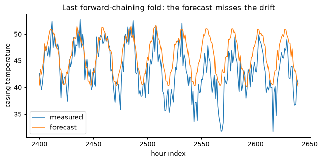
Xtr, Xte, ytr, yte = train_test_split(
    X_bc, y_bc, test_size=0.25, random_state=0, stratify=y_bc)
logreg = make_pipeline(StandardScaler(), LogisticRegression(C=1)).fit(Xtr, ytr)
knn15 = make_pipeline(StandardScaler(), KNeighborsClassifier(15)).fit(Xtr, ytr)
ok_a = (logreg.predict(Xte) == yte).astype(float)       # 1 where model A is right
ok_b = (knn15.predict(Xte) == yte).astype(float)
n = len(yte)
print(f"test cases {n}; errors: logistic {int(n - ok_a.sum())}, "
      f"15-NN {int(n - ok_b.sum())}")
print(f"accuracy: logistic {ok_a.mean():.3f}, 15-NN {ok_b.mean():.3f}")

R = 2000
rng = np.random.default_rng(0)
idx = rng.integers(0, n, size=(R, n))                   # shared by both models
acc_a, acc_b = ok_a[idx].mean(axis=1), ok_b[idx].mean(axis=1)
for name, acc in (("logistic", acc_a), ("15-NN", acc_b)):
    lo, hi = np.percentile(acc, [2.5, 97.5])
    print(f"{name:9s} 95% interval [{lo:.3f}, {hi:.3f}]")
test cases 143; errors: logistic 2, 15-NN 7
accuracy: logistic 0.986, 15-NN 0.951
logistic  95% interval [0.965, 1.000]
15-NN     95% interval [0.909, 0.986]
The two intervals overlap, which is often read as “no significant difference”. That reading is wrong in general: the two accuracies are computed on the same cases, the cases that are easy for one model are mostly easy for the other, so the errors are positively correlated and the difference is determined more precisely than either accuracy. The paired bootstrap resamples the difference case by case; its histogram is the lab’s version of the right panel of Figure 1.14.
diff = acc_a - acc_b
lo, hi = np.percentile(diff, [2.5, 97.5])
print(f"observed difference {ok_a.mean() - ok_b.mean():.3f}")
print(f"paired 95% interval [{lo:.3f}, {hi:.3f}]")
print(f"fraction of replicates with difference <= 0: {np.mean(diff <= 0):.4f}")

n_a_only = int(np.sum((ok_a == 1) & (ok_b == 0)))       # A right, B wrong
n_b_only = int(np.sum((ok_a == 0) & (ok_b == 1)))       # A wrong, B right
print(f"discordant cases: A right/B wrong {n_a_only}, A wrong/B right {n_b_only}")
print(f"chance a resample contains none of the {n_a_only} cases: "
      f"{((n - n_a_only) / n) ** n:.4f}")

fig, ax = plt.subplots(figsize=(6, 3.5))
ax.hist(diff, bins=30, color="tab:blue", edgecolor="white")
ax.axvline(0, color="k", ls="--", label="no difference")
ax.set_xlabel("accuracy(logistic) - accuracy(15-NN) on a bootstrap resample")
ax.set_ylabel("number of replicates")
ax.set_title("Paired bootstrap of the accuracy difference (R = 2000)")
ax.legend()
plt.show()
observed difference 0.035
paired 95% interval [0.007, 0.070]
fraction of replicates with difference <= 0: 0.0065
discordant cases: A right/B wrong 5, A wrong/B right 0
chance a resample contains none of the 5 cases: 0.0062
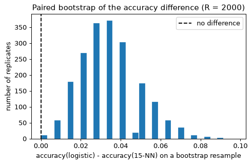
The paired interval excludes zero. The replicates show why: the difference can be zero or negative only if a resample draws none of the five cases on which the models disagree, and the probability of that is (138/143)^{143}.
Step 7: McNemar’s exact test, and why the bootstrap and the test disagree
Only the discordant cases carry information about the difference: where both models are right, or both are wrong, they say nothing about which is better. Under the null hypothesis that the two models are equally accurate, each discordant case is equally likely to go either way, so the number of cases in which A alone is right is binomial with n_{10} + n_{01} trials and success probability 0.5. McNemar’s exact test is the binomial test on that count. Here n_{10} counts the cases A gets right and B wrong, and n_{01} the reverse.
The familiar \chi^2 form, (n_{10} - n_{01})^2/(n_{10} + n_{01}), approximates the exact test for large counts. With few discordant cases it overstates the evidence. Here are all three.
n10, n01 = n_a_only, n_b_only
exact = binomtest(n10, n10 + n01, 0.5).pvalue
chi_plain = (n10 - n01) ** 2 / (n10 + n01)
chi_corrected = (abs(n10 - n01) - 1) ** 2 / (n10 + n01)
print(f"discordant counts n10 = {n10}, n01 = {n01}")
print(f"exact binomial test        p = {exact:.4f}")
print(f"chi-square {chi_plain:.1f}              p = {chi2.sf(chi_plain, 1):.3f}")
print(f"corrected chi-square {chi_corrected:.1f}    p = {chi2.sf(chi_corrected, 1):.3f}")
discordant counts n10 = 5, n01 = 0
exact binomial test        p = 0.0625
chi-square 5.0              p = 0.025
corrected chi-square 3.2    p = 0.074
The methods give different answers to “is the difference of 0.035 real?”. The paired bootstrap says yes, and so does the plain \chi^2 (p = 0.025). The exact test, which is the correct one for these counts, does not reject at 5% (p = 0.0625); the continuity-corrected \chi^2 agrees with it in verdict. They disagree because there is so little to decide on. The bootstrap resamples the observed cases, and with five discordant cases and none the other way, every resample that contains at least one of them has a positive difference, so the interval cannot straddle zero. It treats the sample’s five-to-zero split as if it were the truth, which understates the uncertainty when the count is that small. A five-to-zero split is also not improbable under a fair coin: it happens with probability 2 \times (1/2)^5 = 0.0625.
The honest report is the difference (0.035, five cases in 143), the discordant counts (5 and 0) and the exact p-value (0.0625), with the statement that the data suggest logistic regression is better but 143 cases are too few to be sure. Reporting only “the paired bootstrap interval excludes zero” would be a correct statement of a misleading result. Decide on the exact test before looking at the counts, not after.
Step 8: the summary table
# values copied from Steps 2 to 5 above
table = [
    ("feature selection before CV", "0.87", "0.50", "selection inside the pipeline"),
    ("scaler before CV", "0.9789", "0.9789", "scaler inside the pipeline (free)"),
    ("rows of one specimen split", "0.95 / 1.00", "0.63 / 0.64", "GroupKFold by specimen"),
    ("shuffled time series (RMSE)", "2.33", "4.09", "TimeSeriesSplit with a gap"),
]
print(f"{'case':30s} {'leaky':>12s} {'honest':>12s}   the fix")
for case, leaky_score, honest_score, fix in table:
    print(f"{case:30s} {leaky_score:>12s} {honest_score:>12s}   {fix}")
case                                  leaky       honest   the fix
feature selection before CV            0.87         0.50   selection inside the pipeline
scaler before CV                     0.9789       0.9789   scaler inside the pipeline (free)
rows of one specimen split      0.95 / 1.00  0.63 / 0.64   GroupKFold by specimen
shuffled time series (RMSE)            2.33         4.09   TimeSeriesSplit with a gap
What you should see
- Selecting features on all the data manufactures about 0.87 accuracy from pure noise; inside the pipeline the score returns to chance, about 0.50, for every seed.
- Standardising on all the data changes nothing measurable for the breast-cancer data: the leak exists and is negligible. The fix is free, so make it anyway.
- Split by row, both models recognise specimens rather than learn the property. Split by specimen, both are near chance with a wide spread, which is the honest picture of 40 specimens and a weak signal.
- The shuffled time-series score is at the noise floor because the forest interpolates the drift from neighbouring hours. Forward chaining shows that it cannot forecast the drift.
- Separate intervals overlap while the paired interval excludes zero, so comparisons need paired methods. McNemar’s exact test (p = 0.0625) does not reject at 5%: with five discordant cases the bootstrap interval is too narrow. The honest summary is the difference, the counts, and the exact p-value.
Try this
- Selection bias in model choice. On pure noise with
Xof shape(100, 50), score 200 random subsets of 5 features by 5-fold cross-validation and keep the best: it reaches about 0.67. Then wrap the search in an outer 5-fold loop (nested cross-validation: choose the subset inside each outer training part, score it on the outer test part) and see the score fall to about 0.56. (Those are the values for data drawn withdefault_rng(0); seeds 1 and 2 give 0.70 and 0.60, 0.64 and 0.54, so the gap of about 0.1 is the stable part.) The best of many noisy scores is an optimistic estimate of its own quality. This takes about 20 seconds. - Cluster bootstrap. For leak 2, resample specimens rather than rows and compare the width of the interval with the row bootstrap’s. The rows of a specimen are not independent, so the row bootstrap is too narrow.
- Target leakage. Add a column equal to the label plus small noise (a “result code” recorded after the outcome) and watch every model become brilliant under every splitting scheme. Splitting cannot repair a feature that is not available at prediction time; only knowing what the feature means can.
- The seed lottery. Repeat Step 6 with
random_state1 to 5 in the split. How often is logistic regression better? What happens to the discordant counts and the exact p-value?
Lab 5 — Fitting a hyperelastic material model
Goal. Fit the neo-Hookean coefficient c_1 of a soft hydrogel to a synthetic compression test by weighted least squares, check the formula for its uncertainty against a Monte Carlo experiment, and then watch a fit that is clean inside its range fail outside it. You detect the misfit from the residuals, fit the Gent model (which has a parameter inside a denominator and so needs nonlinear least squares), look at how its two parameters trade off against each other, and write the input checks that make a fitting routine refuse what it cannot honour. The background is Section 12; the least-squares and uncertainty formulas are from Section 2 and Section 5. The data are synthetic so that every number can be reproduced. Everything runs on a laptop CPU in a few seconds and needs no download.
Step 1: the model and the synthetic test
Under uniaxial stretch \lambda (the deformed length over the original, so compression has \lambda < 1), an incompressible neo-Hookean solid has nominal stress
The Gent model stiffens as the polymer chains approach their limit of extensibility:
where \beta = 1/J_m, and \beta = 0 recovers neo-Hookean. The “true” material in this lab is Gent with c_1 = 10 kPa and \beta = 0.2. The test has 16 stretches \lambda = 1 - 0.025k for k = 1, \dots, 16 (strains of 2.5% to 40%). Each point has a recorded standard uncertainty \sigma_i = 0.05\ \text{kPa} + 0.02\,|P_{\text{true},i}|, a small floor plus 2% of the reading, and the measurement is the true stress plus Gaussian noise of that size. Compression stresses are negative in this convention.
import numpy as np
import matplotlib.pyplot as plt
from scipy.optimize import least_squares
from scipy.stats import chi2

np.random.seed(0)

def g(lam):
    return lam - lam ** -2.0

def i1_minus_3(lam):
    return lam ** 2 + 2.0 / lam - 3.0

def p_neo_hookean(lam, c1):
    return 2.0 * c1 * g(lam)

def p_gent(lam, c1, beta):
    return 2.0 * c1 * g(lam) / (1.0 - beta * i1_minus_3(lam))

k = np.arange(1, 17)
lam = 1.0 - 0.025 * k                                   # compression: 0.975 ... 0.600
p_true = p_gent(lam, 10.0, 0.2)
sigma = 0.05 + 0.02 * np.abs(p_true)                    # kPa, recorded with each point
p_meas = p_true + sigma * np.random.default_rng(1).normal(size=16)

print(" k  stretch  stress (kPa)  sigma (kPa)")
for ki, li, pi, si in zip(k, lam, p_meas, sigma):
    print(f"{ki:2d}   {li:.3f}   {pi:9.2f}    {si:8.3f}")
 k  stretch  stress (kPa)  sigma (kPa)
 1   0.975       -1.51       0.081
 2   0.950       -3.07       0.113
 3   0.925       -4.84       0.148
 4   0.900       -6.98       0.185
 5   0.875       -8.51       0.224
 6   0.850      -10.73       0.267
 7   0.825      -13.33       0.313
 8   0.800      -15.48       0.364
 9   0.775      -18.32       0.419
10   0.750      -21.40       0.481
11   0.725      -24.95       0.549
12   0.700      -28.47       0.626
13   0.675      -33.70       0.713
14   0.650      -38.28       0.813
15   0.625      -44.33       0.928
16   0.600      -49.93       1.061
The stress runs from -1.51 kPa at 2.5% strain to -49.93 kPa at 40%, and the recorded uncertainty grows with it. That is why the fit must be weighted: an unweighted fit would let the large-stress points, which have the largest absolute noise, dominate.
Step 2: refuse what cannot be honoured
A fitting routine that always returns a number is dangerous, because a number looks like a result.
Before fitting, check_inputs rejects a missing or non-positive uncertainty (weighted least
squares has no meaning without one), stretches on the wrong side of 1 for the declared loading
direction, and stresses whose sign contradicts that direction. After fitting, the routine also
refuses a non-positive stiffness, since that is not a material. Each refusal says why.
def check_inputs(lam, p, sigma, direction):
    lam, p = np.asarray(lam, float), np.asarray(p, float)
    if direction not in ("compression", "tension"):
        raise ValueError(f"direction must be compression or tension, got {direction!r}")
    if sigma is None:
        raise ValueError("no uncertainty supplied: weighted least squares needs one per point")
    sigma = np.asarray(sigma, float)
    if sigma.shape != p.shape or not np.all(np.isfinite(sigma)) or np.any(sigma <= 0):
        raise ValueError("every point needs a finite, positive uncertainty")
    sign = 1.0 if direction == "compression" else -1.0
    if np.any(sign * (1.0 - lam) <= 0):
        raise ValueError(f"declared {direction}, but some stretches are on the wrong side of 1")
    if np.any(-sign * p <= 0):
        raise ValueError(f"declared {direction}, but some stresses have the wrong sign")

cases = {
    "no uncertainty": (lam, p_meas, None, "compression"),
    "tension stretches, compression declared": (1 + 0.025 * k, p_meas, sigma, "compression"),
    "stress sign flipped": (lam, -p_meas, sigma, "compression"),
}
for name, args in cases.items():
    try:
        check_inputs(*args)
        print(f"{name}: accepted")
    except ValueError as err:
        print(f"{name}: refused -> {err}")
check_inputs(lam, p_meas, sigma, "compression")
print("the real data: accepted")
no uncertainty: refused -> no uncertainty supplied: weighted least squares needs one per point
tension stretches, compression declared: refused -> declared compression, but some stretches are on the wrong side of 1
stress sign flipped: refused -> declared compression, but some stresses have the wrong sign
the real data: accepted
Step 3: weighted least squares in closed form
The likelihood is Gaussian with a different variance for each point, so maximum likelihood is weighted least squares: minimise \sum_i w_i\,(P_i - 2c_1 g_i)^2 with w_i = 1/\sigma_i^2. Setting the derivative to zero gives
the variance following because \hat c_1 is linear in the noisy P_i. Two diagnostics follow: the normalised residuals (P_i - \hat P_i)/\sigma_i, which should look like standard normal draws, and \chi^2_\nu, the sum of their squares divided by the n - 1 degrees of freedom, which should be near 1.
We fit the first 8 points only, strains up to 20%, where a neo-Hookean model is a reasonable
description. The routine also reports the RMS residual divided by the largest measured stress in
the fitted range, a convention that makes fits to different specimens comparable (quote it with the
strain range fitted over). A call to scipy.optimize.least_squares on the weighted residuals should
give the same c_1.
def fit_neo_hookean(lam, p, sigma, direction="compression"):
    check_inputs(lam, p, sigma, direction)
    w, gg = 1.0 / sigma ** 2, g(lam)
    s_gg = np.sum(w * gg ** 2)
    c1 = np.sum(w * p * gg) / (2.0 * s_gg)
    if c1 <= 0:
        raise ValueError(f"fitted stiffness c1 = {c1:.3f} is not positive: not a material")
    resid = p - p_neo_hookean(lam, c1)
    return {
        "c1": c1,
        "se": 1.0 / (2.0 * np.sqrt(s_gg)),
        "norm_resid": resid / sigma,
        "chi2_nu": np.sum((resid / sigma) ** 2) / (len(p) - 1),
        "rms_pct": 100 * np.sqrt(np.mean(resid ** 2)) / np.max(np.abs(p)),
    }

n_fit = 8
fit20 = fit_neo_hookean(lam[:n_fit], p_meas[:n_fit], sigma[:n_fit])
print(f"c1 = {fit20['c1']:.2f} +/- {fit20['se']:.2f} kPa   "
      f"chi2_nu = {fit20['chi2_nu']:.2f}")
print("normalised residuals:", np.round(fit20["norm_resid"], 2))
print(f"RMS residual = {fit20['rms_pct']:.1f}% of the largest stress in range")

def weighted_resid(theta):
    return (p_meas[:n_fit] - p_neo_hookean(lam[:n_fit], theta[0])) / sigma[:n_fit]

check = least_squares(weighted_resid, x0=[5.0])
print(f"least_squares check: c1 = {check.x[0]:.2f}")
c1 = 10.09 +/- 0.10 kPa   chi2_nu = 0.71
normalised residuals: [ 0.51  1.03  0.52 -1.21  0.86  0.2  -1.04 -0.24]
RMS residual = 1.1% of the largest stress in range
least_squares check: c1 = 10.09
The fit recovers c_1 \approx 10.09 kPa against the true 10, with a standard error of 0.10: the estimate is within one standard error of the truth. The normalised residuals scatter within about \pm 1.2 with no pattern, and \chi^2_\nu = 0.71 is consistent with 1 (with 7 degrees of freedom the 95% range of \chi^2_\nu is roughly 0.24 to 2.3). The model is adequate for these data, even though it is not the true model.
Step 4: check the quoted uncertainty by simulation
The formula \operatorname{Var}(\hat c_1) = 1/(4\sum_i w_i g_i^2) assumes the noise is exactly as recorded. Check it by simulation: generate 1,000 new data sets from the fitted curve plus fresh noise with the same \sigma_i, refit each, and compare the spread of the 1,000 coefficients with the formula.
rng = np.random.default_rng(2)
lam8, sig8 = lam[:n_fit], sigma[:n_fit]
curve = p_neo_hookean(lam8, fit20["c1"])
w8, g8 = 1.0 / sig8 ** 2, g(lam8)
refits = []
for _ in range(1000):
    p_new = curve + sig8 * rng.normal(size=n_fit)
    refits.append(np.sum(w8 * p_new * g8) / (2.0 * np.sum(w8 * g8 ** 2)))
refits = np.array(refits)
print(f"Monte Carlo mean {refits.mean():.3f}, SD {refits.std(ddof=1):.4f}")
print(f"formula SD       {fit20['se']:.4f}")
Monte Carlo mean 10.087, SD 0.0999
formula SD       0.0997
The two standard deviations agree to within a percent or so. For a model that is linear in its parameter the formula is exact, so the only disagreement is the simulation’s own sampling error (about 1/\sqrt{2 \times 1000} = 2\% of the SD). The check earns its keep for the nonlinear fit below, where the formula is only a linearisation.
Step 5: extrapolating with a confidence band
The variance of c_1 gives a band on the prediction at any stretch: P(\lambda) = 2c_1 g(\lambda) is linear in c_1, so its standard error is 2|g(\lambda)|\,\mathrm{SE}(c_1), and the 95% band is \pm 1.96 times that. Predict the stress at \lambda = 0.7 (30% strain) and \lambda = 0.6 (40%), beyond the fitted range, and compare with the true material.
for target in (0.7, 0.6):
    pred = p_neo_hookean(target, fit20["c1"])
    half = 1.96 * 2.0 * abs(g(target)) * fit20["se"]
    truth = p_gent(target, 10.0, 0.2)
    print(f"lambda = {target}: predicted {pred:.2f} +/- {half:.2f} kPa, "
          f"true {truth:.2f}, error {100 * (pred / truth - 1):+.1f}%")
lambda = 0.7: predicted -27.06 +/- 0.52 kPa, true -28.82, error -6.1%
lambda = 0.6: predicted -43.96 +/- 0.85 kPa, true -50.57, error -13.1%
The prediction at 40% strain is 13% low, which is 6.6 kPa against a band half-width of 0.85 kPa: about eight times the band. The band is correct for what it claims: it says how much the measurement noise moves c_1. It says nothing about whether the model is right where you are extrapolating, and here it is not, because the true material stiffens (the \beta term) and the neo-Hookean curve cannot. Statistical uncertainty is not model error, and extrapolation is where model error lives.
Step 6: the misfit shows in the residuals
Now fit all 16 points with the same model and look at the residual signs. A correct model leaves residuals of random sign. A wrong model leaves long runs.
fit_all = fit_neo_hookean(lam, p_meas, sigma)
signs = "".join("+" if r > 0 else "-" for r in fit_all["norm_resid"])
print(f"c1 = {fit_all['c1']:.2f} +/- {fit_all['se']:.2f} kPa   "
      f"chi2_nu = {fit_all['chi2_nu']:.1f}")
print("residual signs (k = 1..16):", signs)
print("largest |normalised residual|:", f"{np.max(np.abs(fit_all['norm_resid'])):.1f}")
c1 = 10.55 +/- 0.06 kPa   chi2_nu = 4.5
residual signs (k = 1..16): ++++++++++------
largest |normalised residual|: 3.8
The coefficient has moved to about 10.55 and its standard error has fallen to 0.06, so the estimate looks more precise, while \chi^2_\nu = 4.5 is far from 1 and the signs come in two runs, ten of one sign and six of the other. With 15 degrees of freedom the 95% upper limit of \chi^2_\nu is about 1.7, so the fit is rejected. The smaller standard error is not reassuring: more data of the same kind shrinks the statistical error of a wrong model without bringing it closer to the truth.
Step 7: the Gent model by nonlinear least squares
P_\text{Gent} is linear in c_1 but not in \beta, so there is no closed form. Use
least_squares on the weighted residuals, starting from (5, 0), with bounds c_1 \ge 0 and
0 \le \beta < 1/\max(I_1 - 3) (beyond that bound the denominator reaches zero inside the data)
and x_scale="jac", so that parameters of different magnitude are treated evenly.
The uncertainty is the linearisation of the problem at the solution: with \mathbf{J} the Jacobian of the weighted residuals with respect to the parameters, \operatorname{Cov}(\hat\theta) \approx (\mathbf{J}^\top\mathbf{J})^{-1}. That is the same formula as in the closed form, with \mathbf{J} in place of the design matrix. We fit the full range and the 20% range, and check the standard errors by Monte Carlo.
def fit_gent(lam, p, sigma):
    check_inputs(lam, p, sigma, "compression")
    beta_max = (1.0 - 1e-6) / np.max(i1_minus_3(lam))

    def weighted_resid(theta):
        return (p - p_gent(lam, theta[0], theta[1])) / sigma

    sol = least_squares(weighted_resid, x0=[5.0, 0.0],
                        bounds=([0.0, 0.0], [np.inf, beta_max]), x_scale="jac")
    cov = np.linalg.inv(sol.jac.T @ sol.jac)
    se = np.sqrt(np.diag(cov))
    return {"theta": sol.x, "se": se, "cov": cov,
            "corr": cov[0, 1] / (se[0] * se[1]),
            "chi2_nu": 2.0 * sol.cost / (len(p) - 2)}

gent_all = fit_gent(lam, p_meas, sigma)
gent_20 = fit_gent(lam[:n_fit], p_meas[:n_fit], sigma[:n_fit])
for name, f in (("all 16 points ", gent_all), ("first 8 points", gent_20)):
    print(f"{name}: c1 = {f['theta'][0]:.2f} +/- {f['se'][0]:.2f}   "
          f"beta = {f['theta'][1]:.3f} +/- {f['se'][1]:.3f}   "
          f"corr = {f['corr']:.2f}   chi2_nu = {f['chi2_nu']:.2f}")

# Monte Carlo check of the linearised standard errors, full range
rng = np.random.default_rng(3)
curve = p_gent(lam, *gent_all["theta"])
draws = np.array([fit_gent(lam, curve + sigma * rng.normal(size=16), sigma)["theta"]
                  for _ in range(300)])
print(f"Monte Carlo SDs (300 refits): c1 {draws[:, 0].std(ddof=1):.3f}, "
      f"beta {draws[:, 1].std(ddof=1):.3f}")
all 16 points : c1 = 9.95 +/- 0.10   beta = 0.208 +/- 0.024   corr = -0.78   chi2_nu = 0.40
first 8 points: c1 = 9.95 +/- 0.18   beta = 0.208 +/- 0.210   corr = -0.83   chi2_nu = 0.67
Monte Carlo SDs (300 refits): c1 0.099, beta 0.025
On all 16 points the Gent fit recovers both parameters (c_1 \approx 9.95, \beta \approx 0.21; true 10 and 0.2) with \chi^2_\nu = 0.40, which is a good fit, indeed slightly better than the noise allows: with 14 degrees of freedom a \chi^2_\nu this low has a probability of about 2.5% under a correct model. Read it as a chance draw from one seed, not as a property of the method. The linearised standard errors agree with the Monte Carlo ones.
The two parameters are strongly negatively correlated, about -0.78: a larger \beta stiffens the curve at large strain, and a smaller c_1 compensates at small strain. Fitted to only the first 8 points, \beta is 0.21 \pm 0.21: consistent with the truth, and also with zero. Data that never reach the strains where \beta matters cannot determine it, and the correlation is higher (about -0.83).
Step 8: the loading direction is part of the model
A subtler error than a wrong model form is reading the experiment wrongly. Suppose the compression test is entered as a tension test: \lambda = 1 + \text{strain} and stress |P|. The checks pass for a declared tension, and the model fits a coefficient.
strain = 1.0 - lam
tension_20 = fit_neo_hookean(1.0 + strain[:8], np.abs(p_meas[:8]), sigma[:8],
                             direction="tension")
tension_5 = fit_neo_hookean(1.0 + strain[:2], np.abs(p_meas[:2]), sigma[:2],
                            direction="tension")
correct_5 = fit_neo_hookean(lam[:2], p_meas[:2], sigma[:2])
print(f"20% strain: tension reading c1 = {tension_20['c1']:.2f} kPa "
      f"({100 * (tension_20['c1'] / fit20['c1'] - 1):+.1f}%), "
      f"chi2_nu = {tension_20['chi2_nu']:.1f}")
print(f" 5% strain: tension reading c1 = {tension_5['c1']:.2f} kPa "
      f"({100 * (tension_5['c1'] / correct_5['c1'] - 1):+.1f}%), "
      f"chi2_nu = {tension_5['chi2_nu']:.2f}")
20% strain: tension reading c1 = 12.97 kPa (+28.5%), chi2_nu = 20.7
 5% strain: tension reading c1 = 10.60 kPa (+8.7%), chi2_nu = 0.38
Over 20% strain the misread fit gives c_1 = 12.97 kPa, 28.5% too high, and \chi^2_\nu = 20.7 announces the problem. Over the first 5% only (two points) the misread fit is clean (\chi^2_\nu = 0.38) and still 8.7% high. At small strain g(1-\epsilon) \approx -3\epsilon - 3\epsilon^2 and g(1+\epsilon) \approx 3\epsilon - 3\epsilon^2 have the same magnitude at first order and differ only at second order, which the noise hides. A wrong model can fit well when the data cannot tell the difference, and a good \chi^2_\nu is not evidence that the model is correct.
Step 9: the plots
Three figures, the lab’s versions of Figures 1.16 to 1.18 in Section 12. First, the data with error bars, the 20% neo-Hookean fit and its extrapolation with the 95% band, and the Gent fit.
fine = np.linspace(0.6, 0.99, 200)
c1_hat, se_c1 = fit20["c1"], fit20["se"]
band = 1.96 * 2.0 * np.abs(g(fine)) * se_c1
fig, ax = plt.subplots(figsize=(7, 4.5))
ax.errorbar(1 - lam, p_meas, yerr=sigma, fmt="o", ms=4, capsize=2, color="k",
            label="measured, $\\pm\\sigma_i$")
ax.plot(1 - fine, p_neo_hookean(fine, c1_hat), color="tab:red",
        label="neo-Hookean fitted to strains up to 20%")
ax.fill_between(1 - fine, p_neo_hookean(fine, c1_hat) - band,
                p_neo_hookean(fine, c1_hat) + band, color="tab:red", alpha=0.25,
                label="95% band (noise only)")
ax.plot(1 - fine, p_gent(fine, *gent_all["theta"]), color="tab:blue",
        label="Gent fitted to all 16 points")
ax.axvline(0.2, color="grey", ls=":")
ax.set_xlabel("compressive strain $1 - \\lambda$")
ax.set_ylabel("nominal stress (kPa)")
ax.set_title("Neo-Hookean fit: clean to 20% strain, wrong beyond it")
ax.legend(fontsize=8)
plt.show()
Second, the normalised residuals of the models on all points. Dashed lines mark \pm 2.
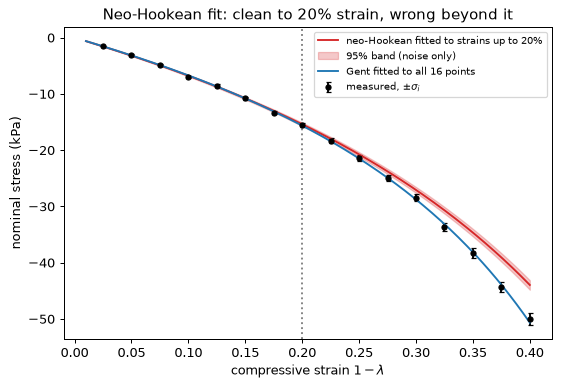
resid_nh20 = (p_meas - p_neo_hookean(lam, fit20["c1"])) / sigma
resid_nh_all = fit_all["norm_resid"]
resid_gent = (p_meas - p_gent(lam, *gent_all["theta"])) / sigma
fig, ax = plt.subplots(figsize=(7, 3.8))
ax.plot(1 - lam, resid_nh20, "o-", color="tab:red", label="neo-Hookean, fitted to 20%")
ax.plot(1 - lam, resid_nh_all, "s-", color="tab:orange",
        label="neo-Hookean, all 16 points")
ax.plot(1 - lam, resid_gent, "^-", color="tab:blue", label="Gent, all 16 points")
for level in (-2, 0, 2):
    ax.axhline(level, color="grey", ls="--" if level else "-", lw=0.8)
ax.set_xlabel("compressive strain $1 - \\lambda$")
ax.set_ylabel("normalised residual $(P_i - \\hat P_i)/\\sigma_i$")
ax.set_title("Residuals: runs of one sign reveal the wrong model")
ax.legend(fontsize=8)
plt.show()
Third, the joint 95% confidence ellipses of (c_1, \beta) for the two strain ranges. The ellipse is \{\theta : (\theta - \hat\theta)^\top \mathrm{Cov}^{-1} (\theta - \hat\theta) \le \chi^2_{2,\,0.95}\}, drawn by mapping the unit circle through the eigen-decomposition of the covariance.
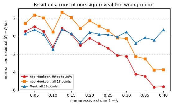
def ellipse(theta_hat, cov, level=0.95, points=200):
    vals, vecs = np.linalg.eigh(cov)
    angle = np.linspace(0, 2 * np.pi, points)
    circle = np.stack([np.cos(angle), np.sin(angle)])
    radius = np.sqrt(chi2.ppf(level, 2))
    return theta_hat[:, None] + radius * vecs @ (np.sqrt(vals)[:, None] * circle)

fig, ax = plt.subplots(figsize=(6, 4.5))
for f, label, colour in ((gent_all, "all 16 points (to 40% strain)", "tab:blue"),
                         (gent_20, "first 8 points (to 20% strain)", "tab:red")):
    xy = ellipse(f["theta"], f["cov"])
    ax.plot(xy[0], xy[1], color=colour, label=label)
    ax.plot(*f["theta"], "o", color=colour)
ax.plot(10.0, 0.2, "k*", ms=10, label="true value")
ax.set_xlabel("$c_1$ (kPa)")
ax.set_ylabel("$\\beta$")
ax.set_title("95% confidence ellipses of the Gent parameters")
ax.legend(fontsize=8)
plt.show()
What you should see
- Inside its range the neo-Hookean fit is clean and precise to 1%. Outside it the prediction at 40% strain is 13% low, about eight times its own band: the interval measures noise, not model error.
- Long runs of same-signed residuals and \chi^2_\nu well above 1 reveal the wrong model once the data reach the strains where the models differ. The standard error of the wrong model shrinks as data are added.
- Linearised uncertainties agree with Monte Carlo for this well-conditioned fit. Jointly fitted parameters are correlated, and \beta is undetermined by data that never exercise it: the ellipse for the 20% range is far larger than the full-range one and extends to \beta = 0.
- The loading direction is part of the model. Misreading it gives 28.5% error over 20% strain, and over a small range the residuals do not betray it.
Try this
- Another model. Fit Mooney–Rivlin, P = 2(\lambda - \lambda^{-2})(c_1 + c_2/\lambda), which is linear in (c_1, c_2) (a two-column weighted least squares), and compare its extrapolation to 40% strain with Gent’s. What does \chi^2_\nu say, and what does the extrapolation band say?
- Experimental design. With only 8 points, choose the stretches that minimise the standard error of \beta (try all eight in [0.6, 0.8] against the evenly spaced design) and recompute. Then argue from the result where the next test should put its points.
- Unknown noise. Replace the recorded \sigma_i by a single unknown \sigma estimated from the residuals, \hat\sigma^2 = \sum_i r_i^2/(n - p), and compare the parameter intervals. When would this be the only option, and what does it cost you?
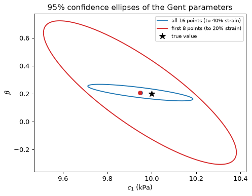
Exercises
Fifteen exercises, graded by the effort they ask for. A one-star exercise (★) is conceptual and takes about five minutes: answer it in words, in a few sentences. A two-star exercise (★★) is a derivation or a calculation of ten to twenty minutes, to be done on paper with a calculator. The one three-star exercise (★★★) is a coding project of about 25 minutes. The total is 130 minutes. The study plan places each exercise after the reading it tests, so that no reading block runs on for long without something to do.
Attempt every exercise before you open its solution. The solutions are hidden until you open them, and they are written to be read in full: they show every step, say why the step is taken, and give the numbers, each of which was computed and checked. If your answer differs from the solution’s, find the first line where the two part company before you read on. A wrong number with a correct method is usually a slip; a correct number reached by a different method is worth comparing with the solution’s, because the difference often shows an assumption.
The five ingredients. Write down the five ingredients of Section 1 (data, model, loss, optimiser, evaluation) for
(a) a linear trendline fitted in a spreadsheet to a strain-gauge calibration, gauge voltage against applied strain; and
(b) a k-nearest-neighbour classifier (k = 5) that labels weld radiographs as acceptable or defective from 20 measured features.
For (b), which ingredient is degenerate, and what does that imply about where its errors come from?
Show solution
(a) The trendline.
- Data. Pairs (applied strain, gauge voltage) from one calibration run, drawn from a distribution P that is the gauge in its calibration set-up. What the gauge will meet in service, in temperature, strain range and lead-wire length, is a different distribution, and the calibration says nothing about it.
- Model. A line, \text{voltage} = a + b\cdot\text{strain}, two parameters. The calibration is used in reverse, to turn a measured voltage into a strain, so the fitted line is inverted at the point of use. The applied strain is set by the rig and known far better than the voltage is, which is why voltage is the variable on the vertical axis: the loss treats the vertical variable as the noisy one.
- Loss. Squared error, which is the right choice if the voltage noise is roughly Gaussian with the same spread at every strain (Section 5).
- Optimiser. The closed form, the normal equations (Section 2). The spreadsheet solves them for you.
- Evaluation. Residuals at check points that were not used in the fit, or a second calibration run. The R^2 that the spreadsheet prints is computed on the fitted points: it is a training score, and a two-parameter line cannot overfit much, but a trendline with six parameters would raise it for free.
(b) The k-NN classifier.
- Data. Labelled radiographs from past inspections. P is welds of this type from this process, so the classifier is only as good as the stored examples are typical of tomorrow’s welds.
- Model. The majority label among the five stored examples nearest to the new weld in the 20-dimensional feature space. Its “parameters” are the stored data themselves, plus the hyperparameters k and the distance (including how each feature is scaled).
- Loss. The 0–1 loss, used only to compare settings of k and the scaling on validation data. Nothing is minimised by training.
- Optimiser. None. “Training” is storing the data, so this is the degenerate ingredient.
- Evaluation. Held-out welds, split by weld or by production batch, never by radiograph if one weld has several.
What the degenerate optimiser implies. There is no optimisation to go wrong, so none of the errors come from a failure to converge, and there is no training curve to inspect. Everything rides on the data and on the distance. The errors come from unrepresentative stored examples, from features that are irrelevant to the defect but count equally in the distance, from features on different scales, and from a space of 20 dimensions in which “near” carries little meaning (Section 11). A second consequence is that the training error is useless: with k = 1 every stored point is its own nearest neighbour, so the training error is zero by construction, and with k = 5 it is nearly so. Only held-out data tell you anything.
Coding a categorical input. A linear model predicts tensile strength from material grade, one of {steel, aluminium, titanium}.
(a) What does coding the grade as 1, 2, 3 assume?
(b) You one-hot encode the grade into three columns and keep the column of ones for the intercept. Show that \mathbf{X}^\top\mathbf{X} is singular, and say what happens to the fitted weights and to the predictions.
(c) Give two fixes.
Show solution
(a) A single column holding 1, 2, 3 gives the grade one weight w, so the model adds w to the prediction when the code goes up by one, whichever grade it starts from. That assumes an order (steel < aluminium < titanium) and equal spacing: aluminium’s effect must lie exactly halfway between steel’s and titanium’s. Nothing about the three materials justifies either. Whatever the data say, a line through the codes predicts the middle grade as the average of its predictions for the other two. If the true strengths were, say, 400, 300 and 900 MPa, that prediction for the middle grade would be badly wrong.
(b) Each row of the one-hot design has a 1 in the intercept column and a single 1 in one of the three grade columns, so in every row the three grade columns sum to the intercept column. Take \mathbf{v} = (-1, 1, 1, 1) over (intercept, steel, aluminium, titanium). Then every row of \mathbf{X}\mathbf{v} is -1 + 1 = 0, so \mathbf{X}\mathbf{v} = \mathbf{0}, and therefore \mathbf{X}^\top\mathbf{X}\mathbf{v} = \mathbf{X}^\top\mathbf{0} = \mathbf{0}. A non-zero vector that the matrix maps to zero is an eigenvector with eigenvalue 0: \mathbf{X}^\top\mathbf{X} is singular, the normal equations have no unique solution, and (\mathbf{X}^\top\mathbf{X})^{-1} does not exist. This is the dependent-columns case of Section 2, and it has a name, the dummy-variable trap.
What this does to the fit: if \mathbf{w} solves the normal equations, so does
\mathbf{w} + t\mathbf{v} for every t, because \mathbf{X}(\mathbf{w} + t\mathbf{v}) =
\mathbf{X}\mathbf{w}. Raising the intercept by t and lowering all three grade weights by t
changes nothing. So the weights are not identified: any of them can take any value, provided the
others compensate, and a statement such as “titanium adds 493 MPa” has no meaning on its own.
The predictions are identified, because they are the orthogonal projection of \mathbf{y} onto
the column space, which does not depend on which basis of that space you chose; here each
grade’s prediction is the mean strength of that grade’s specimens. Library solvers handle the
singularity in their own way: np.linalg.lstsq returns the solution of smallest norm.
A numerical check, with 12 synthetic specimens, four per grade:
import numpy as np

rng = np.random.default_rng(0)
grade = np.repeat([0, 1, 2], 4)                      # 4 specimens per grade
strength = np.array([400.0, 300.0, 900.0])[grade] + rng.normal(0, 10, 12)  # MPa

X = np.column_stack([np.ones(12), np.eye(3)[grade]])   # intercept + one-hot grade
print("columns:", X.shape[1], " rank:", np.linalg.matrix_rank(X))
print("eigenvalues of X^T X:", np.round(np.linalg.eigvalsh(X.T @ X), 2))

v = np.array([-1.0, 1.0, 1.0, 1.0])
print("largest entry of X v:", np.abs(X @ v).max())

w_min = np.linalg.lstsq(X, strength, rcond=None)[0]    # minimum-norm solution
w_shift = w_min + 50 * v                               # another exact solution
print("same predictions:", np.allclose(X @ w_min, X @ w_shift))
print("weights, minimum norm:", np.round(w_min, 1))
print("weights, shifted     :", np.round(w_shift, 1))

X_ref = X[:, [0, 2, 3]]                                # drop the steel column
w_ref = np.linalg.lstsq(X_ref, strength, rcond=None)[0]
print("reference coding:", np.round(w_ref, 1), " same predictions:",
      np.allclose(X_ref @ w_ref, X @ w_min))
columns: 4  rank: 3
eigenvalues of X^T X: [ 0.  4.  4. 16.]
largest entry of X v: 0.0
same predictions: True
weights, minimum norm: [400.2   1.7 -95.  493.5]
weights, shifted     : [350.2  51.7 -45.  543.5]
reference coding: [401.8 -96.7 491.8]  same predictions: True
Four columns but rank 3, and one eigenvalue of \mathbf{X}^\top\mathbf{X} is exactly zero. The two weight vectors differ by 50\,\mathbf{v} and make identical predictions. With steel as the reference category, the weights become interpretable: 401.8 is the mean strength of steel, and the other two are differences from steel (a difference of -96.7 for aluminium, +491.8 for titanium).
(c) Two fixes, with different meanings:
- Remove the redundancy. Drop one grade column and keep the intercept (a reference category: the intercept is that grade’s mean and each remaining weight is a difference from it), or drop the intercept and keep all three columns (each weight is its grade’s mean). The predictions are identical in both cases, and the matrix has full column rank.
- Regularise. A ridge penalty replaces \mathbf{X}^\top\mathbf{X} by \mathbf{X}^\top\mathbf{X} + \lambda N\mathbf{I}, whose eigenvalues are at least \lambda N > 0, so the system has a unique solution (Exercise 8). Among the weight vectors that fit equally well, the penalty picks the one of smallest norm, which settles how the shared constant is split between the intercept and the grade weights. That is a modelling choice, not a neutral one, and it also shrinks the fit slightly.
Step sizes and step counts from eigenvalues. The least-squares Hessian of a two-feature problem has eigenvalues 1 and 25.
(a) What is the largest stable learning rate?
(b) What is the best fixed learning rate, and the error contraction per step it gives?
(c) How many steps reduce the error by a factor of 10^6 at the best rate, and at \eta = 1/\lambda_{\max}?
(d) After standardisation the eigenvalues are 0.8 and 1.2. Repeat (b) and (c).
Show solution
Set-up. On a quadratic with Hessian \mathbf{H}, the error \mathbf{e}_t = \mathbf{w}_t - \mathbf{w}^\ast obeys \mathbf{e}_{t+1} = (\mathbf{I} - \eta\mathbf{H})\mathbf{e}_t (Section 3). In the eigenbasis of \mathbf{H} the components do not interact, and the component along the eigenvector with eigenvalue \lambda_i is multiplied by 1 - \eta\lambda_i at every step. The error as a whole shrinks as fast as its slowest component, so the contraction per step is \rho(\eta) = \max_i |1 - \eta\lambda_i|.
(a) Stability. Every component must shrink, so |1 - \eta\lambda_i| < 1 for every i. For a positive \lambda_i this means 0 < \eta < 2/\lambda_i, and all of them hold when \eta < 2/\lambda_{\max}:
At exactly 0.08 the fast component is multiplied by 1 - 0.08 \cdot 25 = -1: it flips sign and neither grows nor shrinks, so the iteration never converges.
(b) The best fixed rate. Two terms compete: |1 - \eta\lambda_{\min}| falls as \eta grows (the slow direction wants a large step) and |1 - \eta\lambda_{\max}| is what the fast direction suffers once \eta passes 1/\lambda_{\max} (it overshoots, with a negative factor). The best \eta is where the two are equal in magnitude and opposite in sign:
Then \rho = 1 - \eta^\ast\lambda_{\min} = 1 - 0.0769 = 0.9231, and in general
Both components now contract by the same factor in magnitude: the slow one by +0.9231 and the fast one by 1 - 0.0769\cdot 25 = -0.9231.
(c) Step counts. To reduce the error by 10^6 we need \rho^t \le 10^{-6}, that is, t \ge \ln 10^6/(-\ln\rho). With \ln 10^6 = 13.816:
- At the best rate, -\ln 0.9231 = 0.0800, so t \ge 13.816/0.0800 = 172.6: 173 steps.
- At \eta = 1/\lambda_{\max} = 0.04, the factors are 1 - 0.04\cdot 1 = 0.96 for the slow component and 1 - 0.04 \cdot 25 = 0 for the fast one. The slow one decides: -\ln 0.96 = 0.0408, so t \ge 13.816/0.0408 = 338.4: 339 steps.
The best rate roughly halves the count, by giving up the instant convergence of the fast direction in return for a faster slow one. Neither escapes the fact that the count is of order \kappa: for large \kappa, -\ln\rho = \ln\frac{\kappa+1}{\kappa-1} \approx 2/\kappa, so t \approx (\kappa/2)\ln 10^6 (here 12.5 \times 13.8 = 173). A direct simulation of the two components confirms 173 and 339.
(d) After standardisation. Now \kappa = 1.2/0.8 = 1.5.
- \eta^\ast = 2/(0.8 + 1.2) = 1.0.
- The factors are 1 - 1.0\cdot 0.8 = +0.2 and 1 - 1.0\cdot 1.2 = -0.2, so \rho = 0.2, which agrees with (\kappa - 1)/(\kappa + 1) = 0.5/2.5 = 0.2.
- t \ge 13.816/(-\ln 0.2) = 13.816/1.609 = 8.58: 9 steps.
Standardising took the count from 173 to 9, about twenty times fewer, with no change of method and no change in what the model can represent. This is why centring and scaling the features is the cheapest optimisation improvement there is.
Cross-entropy against squared error through a sigmoid.
(a) Show that the gradient of binary cross-entropy with respect to the logit z is \hat p - y, where \hat p = \sigma(z).
(b) Compute the gradient of \tfrac12(\sigma(z) - y)^2 with respect to z.
(c) Evaluate both for a confidently wrong prediction, \hat p = 0.999 with y = 0, and for a confidently right one, \hat p = 0.001 with y = 0.
(d) What do the numbers mean for learning?
Show solution
(a) The loss for one example is \ell = -y\ln\sigma(z) - (1-y)\ln(1-\sigma(z)). The sigmoid has derivative \sigma'(z) = \sigma(z)(1 - \sigma(z)) (differentiate 1/(1 + e^{-z}) and simplify). By the chain rule,
The factor \sigma(1 - \sigma) from the sigmoid cancels the denominators from the logarithm. That cancellation is the reason cross-entropy and the sigmoid are used together.
(b) Write \ell_2 = \tfrac12(\sigma(z) - y)^2. Then
Nothing cancels: the sigmoid’s derivative stays as an extra factor.
(c) The numbers. With y = 0 the two gradients are \hat p and \hat p\cdot\hat p(1 - \hat p) = \hat p^2(1-\hat p).
| cross-entropy gradient | squared-error gradient | |
|---|---|---|
| confidently wrong, \hat p = 0.999 | 0.999 | 0.999^2 \times 0.001 = 0.000998 |
| confidently right, \hat p = 0.001 | 0.001 | 0.001^2 \times 0.999 = 9.99\times10^{-7} |
In both rows the ratio is 1/(\hat p(1 - \hat p)) at \hat p = 0.999 or 0.001, which is 1/(0.999 \times 0.001) = 1001: the cross-entropy gradient is about 1,001 times the squared-error one.
(d) What this means. A gradient step moves the logit by an amount proportional to the gradient. Cross-entropy’s gradient \hat p - y is the prediction error itself: it is near 1 when the model is confidently wrong, shrinks smoothly as the model improves, and is near 0 when it is right. The squared-error gradient carries the extra factor \hat p(1 - \hat p), which is near zero at both extremes because the sigmoid is flat there (it saturates). So the model that is most wrong, with its logit at about z = \ln(0.999/0.001) = +6.9 for a negative example, receives almost no signal: its gradient is 0.001, and it learns about a thousand times more slowly than under cross-entropy. At its largest, the squared-error gradient, \hat p^2(1-\hat p), reaches only 4/27 = 0.148 (at \hat p = 2/3), against a cross-entropy gradient that reaches 1.
Cross-entropy also gives the right loss values: -\ln 0.001 = 6.9 for the confidently wrong prediction against \tfrac12(0.999)^2 = 0.5 for squared error, which can never exceed \tfrac12. A loss that cannot tell a mildly wrong prediction from a catastrophic one, and a gradient that vanishes exactly when the model most needs correction, is why classification is trained with cross-entropy (Section 6). The same cancellation, \hat{\mathbf{p}} - \mathbf{y}, holds for softmax, and so for the output layer of a language model.
What an alarm means. A crack detector has recall 0.90 and false-positive rate 0.03, and cracks are present in 2% of inspected parts.
(a) What fraction of flagged parts actually have a crack, and how many false alarms come with each true one?
(b) Show that the odds of a crack given an alarm are the prior odds times TPR/FPR, and use this to find the prevalence at which half the alarms are true.
(c) Every flagged part goes to a second inspection with the same recall and false-positive rate, whose errors are independent of the first’s given the true state. What fraction of twice-flagged parts have a crack, what is the recall of the two stages together, and what fraction of all parts does the second stage inspect?
(d) Which numbers in the vendor’s brochure would have hidden the answer to (a)?
Show solution
(a) Work with fractions of all parts. Let \pi = 0.02 be the prevalence, TPR = 0.90 the recall and FPR = 0.03.
- Cracked parts that are flagged: \text{TPR}\cdot\pi = 0.90 \times 0.02 = 0.0180 of all parts.
- Good parts that are flagged: \text{FPR}\cdot(1-\pi) = 0.03 \times 0.98 = 0.0294 of all parts.
- All flagged: 0.0180 + 0.0294 = 0.0474.
Precision is the cracked fraction of the flagged:
Fewer than four alarms in ten are real. False alarms per true alarm: 0.0294/0.0180 = 1.63.
(b) By Bayes’ rule,
The two probabilities share the denominator P(\text{alarm}), which cancels in the ratio. So the posterior odds are the prior odds multiplied by the likelihood ratio TPR/FPR, which here is 0.90/0.03 = 30. Check on (a): prior odds 0.02/0.98 = 0.0204, times 30 gives 0.612, and odds 0.612 correspond to the probability 0.612/1.612 = 0.380. Matches.
Half the alarms are true when the posterior odds are 1, so \pi/(1-\pi) = \text{FPR}/\text{TPR}, which gives
A detector whose alarms are mostly false at 2% prevalence is mostly right at 3.2% and above: the same classifier, with the same recall and false-positive rate, is a different tool in a different population (Section 7, the base rate).
(c) The second stage sees only parts that the first flagged, so the prior odds it faces are the posterior odds of the first stage, 0.612. Its alarm multiplies them by the likelihood ratio again, because the two errors are independent given the true state:
Equivalently, directly: cracked and flagged twice 0.90^2\times 0.02 = 0.0162; good and flagged twice 0.03^2\times 0.98 = 0.000882; the ratio 0.0162/(0.0162 + 0.000882) = 0.948.
- Recall of the two stages together: a crack must be caught by both, so 0.90 \times 0.90 = 0.81. The second stage costs 9 points of recall (0.90 to 0.81) in exchange for lifting precision from 0.38 to 0.95; false alarms per true alarm fall from 1.63 to 0.000882/0.0162 = 0.054.
- Parts the second stage inspects: those the first flags, 4.74% of all parts.
The independence assumption is optimistic, in both directions. If the two inspections miss the same subtle cracks, the cracks that the first stage flags are the easy ones, which the second stage catches more often than 0.90, so the real combined recall is higher than 0.81. If they raise false alarms on the same awkward but sound parts, the second stage removes fewer of them than the factor of 30 suggests, and the real precision is lower than 0.948. Measure the correlation on real data before relying on the products.
(d) Two numbers hide it. Accuracy: 0.0180 + 0.97\times0.98 = 0.9686, which sounds excellent, and is lower than the 0.98 achieved by a “detector” that never raises an alarm. The accuracy is dominated by the 98% of good parts that are correctly passed. ROC AUC, and any curve plotted against TPR and FPR, because neither depends on prevalence: a brochure that reports them says nothing about how many alarms will be false in your population. A brochure benchmarked on a balanced test set (half cracked) would also show precision 0.90/0.93 = 0.97 for this same detector. What shows (a) is the precision at the deployment prevalence, or the precision–recall curve computed on data with the real mix of cracked and good parts.
AUC by counting pairs. Six test parts receive scores. Defective: 0.9, 0.7, 0.4. Good: 0.8, 0.3, 0.2.
(a) Compute the AUC by counting pairs.
(b) Sweep the threshold downward and list the (FPR, TPR) points of the ROC curve; check that the area under the staircase equals (a).
(c) At threshold 0.5, give precision and recall.
(d) Which single score change would raise the AUC to 1?
Show solution
(a) Counting pairs. The AUC is the probability that a randomly chosen defective part scores higher than a randomly chosen good one (ties counting one half; there are none here). There are 3 \times 3 = 9 defective–good pairs. For each defective part, count the good parts it outscores:
- 0.9 beats 0.8, 0.3 and 0.2: 3 pairs.
- 0.7 beats 0.3 and 0.2 but not 0.8: 2 pairs.
- 0.4 beats 0.3 and 0.2 but not 0.8: 2 pairs.
(b) The ROC curve. Lower the threshold through the scores in decreasing order. A threshold flags every part scoring at or above it. Each defective part passed raises TPR by 1/3; each good part raises FPR by 1/3.
| threshold reaches | part | FPR | TPR |
|---|---|---|---|
| (above 0.9) | none flagged | 0 | 0 |
| 0.9 | defective | 0 | 1/3 |
| 0.8 | good | 1/3 | 1/3 |
| 0.7 | defective | 1/3 | 2/3 |
| 0.4 | defective | 1/3 | 1 |
| 0.3 | good | 2/3 | 1 |
| 0.2 | good | 1 | 1 |
The area under the staircase, taken in vertical strips: for FPR from 0 to 1/3 the height is
1/3, an area \tfrac13\cdot\tfrac13 = 1/9; for FPR from 1/3 to 1 the height is 1, an area
\tfrac23\cdot 1 = 6/9. Total 7/9, which agrees with (a). (The two computations are the same
sum arranged differently: counting pairs by defective part, or by good part.) A machine check with
sklearn.metrics.roc_auc_score returns 0.7778.
(c) Threshold 0.5. The parts scoring at least 0.5 are 0.9 (defective), 0.8 (good) and 0.7 (defective). So TP = 2, FP = 1; the defective part scoring 0.4 is missed, FN = 1; TN = 2.
(d) One change. An AUC of 1 means every defective part outscores every good one, so the three scores 0.9, 0.7, 0.4 must all sit above the three good scores. The only obstacle is the good part scored 0.8, which beats the defective 0.7 and 0.4. Lowering it below 0.4, for example to 0.35, gives AUC 1. Raising the defective 0.4 alone cannot work: to 0.95 it fixes one pair, but the defective 0.7 still sits below the good 0.8, and the AUC becomes only 8/9. (Raising both 0.7 and 0.4 above 0.8 would also work, but that is two changes.) The exercise shows what the AUC measures: it is a statement about the ordering of scores, and a single badly scored good part costs two of the nine pairs.
Shrinkage in one dimension. You estimate a mean \mu from n independent readings of variance \sigma^2, using the shrunk estimator \hat\mu_c = c\,\bar y with 0 \le c \le 1.
(a) Derive its bias^2, variance and mean squared error.
(b) Find the c that minimises the MSE.
(c) Take \sigma = 3 and n = 9. Evaluate c^\ast and its MSE for \mu = 2 and for \mu = 0.5, and compare with the MSE of \bar y.
(d) Why can you not use c^\ast directly in practice? Compute the MSE when the c^\ast for \mu = 0.5 is used but \mu is really 2, and say what this has to do with choosing \lambda by cross-validation.
Show solution
(a) The sample mean \bar y has \mathbb{E}[\bar y] = \mu and \operatorname{Var}(\bar y) = \sigma^2/n (the variance of an average of n independent readings). Multiplying by the constant c:
- \mathbb{E}[\hat\mu_c] = c\mu, so the bias is c\mu - \mu = -(1-c)\mu and \text{bias}^2 = (1-c)^2\mu^2.
- \operatorname{Var}(\hat\mu_c) = c^2\sigma^2/n.
The mean squared error is the sum of the two (the cross term vanishes, as in Section 8):
(b) Write v = \sigma^2/n. Differentiate with respect to c and set the derivative to zero:
The second derivative 2\mu^2 + 2v is positive, so this is a minimum, and c^\ast lies between 0 and 1, so the constraint is not active. Substituting 1 - c^\ast = v/(\mu^2 + v),
Since c^\ast < 1 this is below v = \text{MSE}(1), the MSE of the unbiased \bar y: some bias always pays for itself, and the best c trades it against variance exactly as in the bias–variance decomposition. (The shrink factor has the form of the ridge factor s^2/(s^2 + \lambda N) of Exercise 8. With a Gaussian prior of variance \tau^2 on \mu, as in Section 9, the posterior mean is \tau^2/(\tau^2 + v)\,\bar y, the same form with \tau^2 in place of the unknown \mu^2.)
(c) The numbers. Here v = \sigma^2/n = 9/9 = 1, so \bar y has MSE 1.0 whatever \mu is.
- \mu = 2: c^\ast = 4/(4 + 1) = 0.8. Bias^2 = (0.2)^2\cdot 4 = 0.16, variance 0.8^2\cdot 1 = 0.64, MSE = 0.80 = c^\ast v. A 20% reduction.
- \mu = 0.5: c^\ast = 0.25/(0.25 + 1) = 0.2. Bias^2 = 0.8^2 \cdot 0.25 = 0.16, variance 0.2^2\cdot 1 = 0.04, MSE = 0.20. An 80% reduction.
Shrinking helps most when the signal is small against the noise, because then the unbiased estimate is mostly noise and discarding some of it costs little. (A simulation of 10^6 samples gives 0.800 and 0.200.)
(d) The catch. c^\ast depends on \mu, the very quantity being estimated. Suppose you believe \mu = 0.5 and shrink with c = 0.2, but \mu is really 2:
two and a half times the MSE of the plain mean \bar y (1.0). Shrinkage chosen without evidence, or chosen from the wrong belief, can do real harm: the bias term grows with the square of the distance from the true value, and nothing in the formula warns you.
The remedy is to choose the amount of shrinkage from the data, by estimating the error directly on held-out data, which is what validation and cross-validation do. In ridge regression a larger strength \lambda means a smaller c: a \lambda chosen by cross-validation is an estimate of the unknowable c^\ast, and Lab 3 shows the ridge path and its minimum on noisy data. The estimate is itself noisy, but unlike the guess above it is anchored to the data.
Normal equations and ridge.
(a) Derive the normal equations from the gradient of \mathcal{L}(\mathbf{w}) = \tfrac1N\|\mathbf{X}\mathbf{w} - \mathbf{y}\|^2.
(b) Add the ridge penalty \lambda\|\mathbf{w}\|^2 and show that the system becomes (\mathbf{X}^\top\mathbf{X} + \lambda N\mathbf{I})\mathbf{w} = \mathbf{X}^\top\mathbf{y}.
(c) Using the eigenvalues of \mathbf{X}^\top\mathbf{X}, explain why this system is solvable for every \lambda > 0, even when \mathbf{X} has fewer rows than columns.
(d) If \mathbf{X}^\top\mathbf{X} has eigenvalues 50 and 0.5 and \lambda N = 5, give the shrinkage factor s^2/(s^2 + \lambda N) of each direction and the condition numbers before and after.
Show solution
(a) Expand the squared norm: \|\mathbf{X}\mathbf{w} - \mathbf{y}\|^2 = \mathbf{w}^\top\mathbf{X}^\top\mathbf{X}\mathbf{w} - 2\mathbf{w}^\top\mathbf{X}^\top\mathbf{y} + \mathbf{y}^\top\mathbf{y}. The gradient of a quadratic form \mathbf{w}^\top\mathbf{A}\mathbf{w} with symmetric \mathbf{A} is 2\mathbf{A}\mathbf{w}, the gradient of \mathbf{w}^\top\mathbf{b} is \mathbf{b}, and the last term does not depend on \mathbf{w}, so
At a minimum the gradient is zero: \mathbf{X}^\top\mathbf{X}\mathbf{w} = \mathbf{X}^\top\mathbf{y}. These are the normal equations. (The Hessian is \tfrac2N\mathbf{X}^\top\mathbf{X}, positive semi-definite, so the loss is convex and a point with zero gradient is a global minimum.)
(b) The penalised loss is \mathcal{L}(\mathbf{w}) + \lambda\|\mathbf{w}\|^2, and \nabla_{\mathbf{w}}\lambda\|\mathbf{w}\|^2 = 2\lambda\mathbf{w}. Setting the total gradient to zero:
Multiply by N/2: \mathbf{X}^\top\mathbf{X}\mathbf{w} - \mathbf{X}^\top\mathbf{y} + \lambda N\mathbf{w} = \mathbf{0}, which rearranges to
The factor N appears because \mathcal{L} is the mean loss and the penalty is added to it unscaled; a loss written as a sum would give \lambda\mathbf{I} instead.
(c) \mathbf{X}^\top\mathbf{X} is symmetric, so it has real eigenvalues s_i^2 with orthogonal eigenvectors \mathbf{v}_i, and each is non-negative: s_i^2 = \mathbf{v}_i^\top \mathbf{X}^\top\mathbf{X}\mathbf{v}_i = \|\mathbf{X}\mathbf{v}_i\|^2 \ge 0 (for a unit eigenvector). Adding \lambda N\mathbf{I} adds \lambda N to every eigenvalue and leaves the eigenvectors alone, so the eigenvalues of the ridge matrix are s_i^2 + \lambda N \ge \lambda N > 0. A symmetric matrix whose eigenvalues are all positive is invertible, so the system has exactly one solution for every \lambda > 0.
This holds even when \mathbf{X} has fewer rows than columns (N < d + 1) or dependent columns (Exercise 2). Then \mathbf{X}^\top\mathbf{X} has rank at most N, so at least d + 1 - N eigenvalues are exactly zero and the unpenalised system has infinitely many solutions. The penalty lifts those zeros to \lambda N and picks, among all the weight vectors that fit equally well, the one of smallest norm.
(d) A worked case. In the eigenbasis, ridge multiplies the least-squares component along each direction by s^2/(s^2 + \lambda N). (Derivation: in the basis of the \mathbf{v}_i the system decouples into (s_i^2 + \lambda N)\,\tilde w_i = s_i^2\,\tilde w_i^{\text{LS}}, because \mathbf{X}^\top\mathbf{y} = \mathbf{X}^\top\mathbf{X}\mathbf{w}^{\text{LS}} whenever the least-squares solution exists.) With \lambda N = 5:
- direction with s^2 = 50: 50/55 = 0.909;
- direction with s^2 = 0.5: 0.5/5.5 = 0.091.
The well-determined direction, in which the data fix the weight tightly, keeps 91% of its least-squares value. The poorly determined direction, which the data barely constrain, keeps 9%: ridge removes most of what the data cannot support and little of what they can. The condition number falls from 50/0.5 = 100 to (50 + 5)/(0.5 + 5) = 55/5.5 = 10, so gradient descent on the ridge loss also converges about ten times faster, in the sense of Exercise 3.
Spot the leak. For each set-up say whether there is leakage, of which kind, and how to fix it.
(a) Missing values are imputed with the column mean of the full dataset, then 5-fold cross-validation is run.
(b) Vibration spectra from 12 pumps, 500 per pump, are split 80/20 at random.
(c) Next-day failure is predicted from features that include “hours since last maintenance”, recorded at the end of the day of the failure.
(d) A model is tuned on the test set because the validation set was “too small”.
Show solution
(a) Preprocessing leakage, usually mild. The column means include the values in the rows that
each fold uses for validation, so a little information about the held-out rows reaches the model
through its inputs. For a mean over many rows the effect is small, which is why this leak often
survives unnoticed; for statistics that depend more on individual rows (target encoding, feature
selection by correlation with the label, PCA fitted on everything) it can be large. Fix: put
the imputer inside a Pipeline so that cross-validation fits it on each training fold only:
make_pipeline(SimpleImputer(strategy="mean"), model). The rule is that anything with a fit
step is part of the model.
(b) Group leakage. A random split puts spectra from the same pump on both sides, and a pump’s
spectra resemble each other far more than they resemble another pump’s, so the model can score
well by recognising the pump instead of the fault. The score then says nothing about a pump
the model has never seen, which is the case in use. Fix: split by the unit that will be new
in use: GroupKFold with the pump as the group, or hold out two or three pumps entirely.
A simulation shows the size of the effect. Twelve pumps each have a signature in five features and a “wear” value unrelated to the signature; a 5-nearest-neighbour regressor predicts the wear:
import numpy as np
from sklearn.impute import SimpleImputer
from sklearn.model_selection import GroupKFold, KFold, cross_val_score
from sklearn.neighbors import KNeighborsRegressor
from sklearn.pipeline import make_pipeline

rng = np.random.default_rng(0)
n_pumps, per_pump = 12, 500
pump = np.repeat(np.arange(n_pumps), per_pump)
signature = rng.normal(0, 3, size=(n_pumps, 5))        # each pump's own spectrum
wear = rng.normal(0, 1, n_pumps)                       # unrelated to its spectrum
X = signature[pump] + rng.normal(0, 1, size=(n_pumps * per_pump, 5))
y = wear[pump] + rng.normal(0, 0.2, n_pumps * per_pump)
X[rng.random(X.shape) < 0.05] = np.nan                 # 5% missing values

# (a) the imputer sits inside the pipeline, so each fold fits it on its training rows
model = make_pipeline(SimpleImputer(strategy="mean"), KNeighborsRegressor(5))
score = "neg_root_mean_squared_error"
rmse_random = -cross_val_score(model, X, y, cv=KFold(4, shuffle=True, random_state=0),
                               scoring=score).mean()
rmse_by_pump = -cross_val_score(model, X, y, cv=GroupKFold(4), groups=pump,
                                scoring=score).mean()
print(f"spread of y             : {y.std():.2f}")
print(f"random split, RMSE      : {rmse_random:.2f}")
print(f"split by pump, RMSE     : {rmse_by_pump:.2f}")
spread of y             : 1.12
random split, RMSE      : 0.44
split by pump, RMSE     : 1.72
The random split reports an RMSE of 0.44 against a spread of 1.12 in y: an apparently good model. Split by pump, the RMSE is 1.72, worse than predicting the mean, because the model has nothing to offer for a pump it has not seen. By construction there was never anything to learn. (RMSE is used here and not R^2 because the denominator of R^2 changes with the fold.)
(c) Target leakage, with a temporal flavour. Maintenance performed after the failure resets “hours since last maintenance”, so the value recorded at the end of the failure day encodes the outcome. The feature is not available at the time the prediction would be made, and a model that uses it is predicting the past. Fix: define for every feature the time at which it is known and build the feature table as of the prediction time, with an explicit cut-off. A strong accuracy that collapses when the model runs live is the usual symptom. Checking which feature the model relies on most (and asking why) finds many such leaks.
(d) Test-set reuse. Once the test set has guided a choice (of model, of hyperparameters, of threshold) it has become a validation set, and its score is optimistic by the amount of selection (Section 10). A small validation set is a reason to use cross-validation, not to borrow the test set. Fix: tune by cross-validation on the training data (nested, if the cross-validation score is itself reported), and keep, or collect, a test set that has not been touched, opened once after all decisions are made.
Before believing 98%. A colleague reports 98% accuracy for a model that classifies hazards as controllable or not controllable. List the five questions you ask before believing it, and for each the answer that would make you trust the number.
Show solution
Five questions, each aimed at one way a high accuracy can be empty:
- What is the class balance, and what does the majority-class rule score? If 97% of the hazards are controllable, a model that always answers “controllable” scores 97%, and 98% adds little. Trust if 98% is clearly above the majority baseline, and the baseline is reported beside it.
- What are the confusion matrix and the per-class precision and recall? Accuracy averages over classes weighted by their frequency, so it hides how the rare, costly class is treated. A hazard wrongly called controllable is the dangerous error. Trust if the recall on the “not controllable” class and the precision of the alarms are acceptable for the decision the model supports.
- How was the data split, and were duplicates removed? The same hazard, or near-copies of it across analyses of the same system, on both sides of the split inflates the score (Exercise 9). Trust if the split is by the unit that will be new in use (system, project or hazard scenario, not row), and exact and near duplicates were removed before splitting.
- How many models and settings were tried, and was the test set opened once? The best of many scores is optimistic (Exercise 11), and a test set consulted repeatedly is a validation set. Trust if all choices were made on training data or by cross-validation and the test set was scored once, with the number written down before the look.
- Do the test cases come from the conditions of use, and how many are there? A test set from another industry, an older labelling practice or last year’s systems measures a different problem, and a test set of 100 cases leaves an interval several points wide (Section 10). Trust if the cases resemble the future inputs in kind and in time, and the interval, from a bootstrap for example, is reported and narrow enough to matter.
A sixth question is worth asking when the labels were made by people: how well do the labellers agree with each other? If two engineers agree on 95% of the hazards, a model cannot meaningfully be judged at 98%, since the “ground truth” is itself wrong or contested on that fraction of the cases.
The best of 120. You run a random search over 120 configurations of a gradient-boosting model, score each by 5-fold cross-validation and report the best score.
(a) Why is that score optimistic even if every configuration is equally good?
(b) Does the optimism grow or shrink with (i) more configurations, (ii) more data, (iii) configurations so alike that their scores are nearly identical? One sentence each.
(c) What is the remedy, and why does it work?
Show solution
(a) A cross-validation score is the configuration’s true performance plus noise that comes from the particular folds and the particular data. Picking the best of 120 picks the configuration whose noise happened to be the most favourable, so the maximum is biased upward even when no configuration is better than another. The bias is a property of the selection and of the noise, and it does not need any configuration to be overfitted (Section 10).
(b)
- (i) More configurations: the optimism grows, but slowly. The expected maximum of n independent standard normal draws rises roughly like \sqrt{2\ln n}; simulation gives 1.5 for 10 draws, 2.6 for 120 and 3.3 for 1,200, in units of the noise’s standard deviation. Searching ten times as much adds little, which is also why random search stops paying.
- (ii) More data: the optimism shrinks, because each score’s noise falls like 1/\sqrt{N}, and the selection bias is a multiple of that noise.
- (iii) Nearly identical configurations: the optimism shrinks, because scores that are strongly correlated behave like fewer independent draws, so there is less to pick the luckiest from. (The same folds are shared by all 120 configurations, which already makes their noise correlated, so the figures in (i) are an upper bound.)
(c) Score the chosen configuration on data that played no part in the selection: nested cross-validation (an inner loop that selects, an outer loop that scores the whole procedure, selection included), or a test set opened once after every choice has been made. The selected model is then measured on noise it was not selected for, so its luck, which is independent of that noise, averages out and the score is an honest estimate of the procedure’s performance. The cost of nested cross-validation is the extra fits; the cost of a single test set is that it can be used only once. Lab 4’s extension shows the size of the effect on pure noise, where every configuration is exactly as good as chance.
Forty-seven useless features. A k-nearest-neighbour classifier (k = 5, standardised features) detects bearing faults well from 3 vibration features computed on about 3,000 labelled windows. A new data logger adds 47 further features, most of them unrelated to faults, and the cross-validated accuracy falls although no information was removed.
(a) Give two reasons, both about distances.
(b) Name two remedies.
(c) Why would a gradient-boosted tree ensemble lose much less from the same 47 features?
Show solution
(a) Two reasons.
- Irrelevant features dilute the distance. After standardisation every feature contributes about the same spread to the squared distance. Each of the 47 irrelevant features adds as much squared distance between two random windows as an informative one does, so 47 noise terms swamp 3 signal terms, and the “nearest” neighbours are near in directions that mean nothing. The informative differences are still there; they are just a small part of the total.
- The curse of dimensionality. In 50 dimensions a neighbourhood that holds a fixed fraction of the data has to span most of every feature’s range. A cube holding 1% of uniformly spread data has an edge of 0.01^{1/d} of the range: 0.22 for d = 3, but 0.91 for d = 50 (Section 11). With 3,000 windows, the five nearest are not local at all, and distances between a point and its nearest and its farthest neighbour become nearly equal.
(b) Two remedies.
- Select or reduce features. Choose them by validation, inside the cross-validation folds so that the selection does not leak the labels (Lab 4); or use domain knowledge to keep the features that physics says matter; or reduce dimension with PCA, remembering that PCA keeps directions of large variance, which need not be the ones that carry the fault.
- Learn the distance. Weight the features (for example by validated relevance), or use a model that learns which inputs matter, and keep k-NN for problems with few, well-chosen features.
(c) Why trees cope. Each split of a tree uses one feature and one threshold, chosen from the available features because it reduces the impurity most. An irrelevant feature seldom wins that selection, so it is seldom used, and no step ever combines all 50 features into a single distance. The ensemble therefore ignores most of the noise features instead of averaging over them. They are not free: with 47 candidates per split a noise feature wins by chance now and then, and the trees fit a little noise.
A simulation of the set-up (3,000 windows, three features whose mean shifts with the fault, 47 standard-normal features independent of it) shows the difference:
import numpy as np
from sklearn.ensemble import HistGradientBoostingClassifier
from sklearn.model_selection import StratifiedKFold, cross_val_score
from sklearn.neighbors import KNeighborsClassifier
from sklearn.pipeline import make_pipeline
from sklearn.preprocessing import StandardScaler

rng = np.random.default_rng(0)
n = 3000
fault = rng.integers(0, 2, n)
# three informative features: the mean shifts when a fault is present
signal = rng.normal(size=(n, 3)) + fault[:, None] * np.array([1.2, 0.8, 1.0])
noise = rng.normal(size=(n, 47))                       # 47 unrelated features
cv = StratifiedKFold(5, shuffle=True, random_state=0)

for name, X in [("3 features ", signal), ("50 features", np.hstack([signal, noise]))]:
    knn = make_pipeline(StandardScaler(), KNeighborsClassifier(5))
    boost = HistGradientBoostingClassifier(random_state=0)
    acc_knn = cross_val_score(knn, X, fault, cv=cv).mean()
    acc_boost = cross_val_score(boost, X, fault, cv=cv).mean()
    print(f"{name}: k-NN {acc_knn:.3f}   boosting {acc_boost:.3f}")
3 features : k-NN 0.772   boosting 0.769
50 features: k-NN 0.659   boosting 0.789
The k-NN accuracy falls by 11 points, from 0.77 to 0.66; the boosted trees do not fall at all. (The boosted trees are in fact about two points better with the noise features, in this simulation and in each of the other seeds tried. The exercise does not explain that and it is not a benefit of noise features; the point is only that the trees do not fall.)
Is gradient boosting the baseline to beat? Test the claim that gradient boosting is the
baseline to beat on tabular data. With 5-fold cross-validation using the same folds for every
model (KFold(5, shuffle=True, random_state=0)), compare the RMSE of
- predicting the mean (
DummyRegressor); - ridge (
StandardScaler+RidgeCV(alphas=np.logspace(-3, 3, 13))); - k-NN (
StandardScaler+KNeighborsRegressor(10)); - an RBF support-vector regressor (
StandardScaler+SVR(C=10)); - a random forest (300 trees,
random_state=0); HistGradientBoostingRegressor(random_state=0),
on (a) make_friedman1(n_samples=2000, n_features=10, noise=1.0, random_state=0) and (b)
load_diabetes. Report the mean \pm standard deviation over folds and the fit time. Then
compute the fold-wise RMSE differences between the two best models on each dataset and say
whether the ranking is supported.
Show solution
Plan. Build the six models as pipelines, so that scaling is fitted inside each fold (the
distance-based models and ridge need it; trees do not care). Use one KFold object for every
call, so that each model is scored on exactly the same test folds; that is what makes the
fold-wise differences meaningful. cross_validate with neg_root_mean_squared_error returns
one RMSE per fold. The “two best” are chosen by mean RMSE, and the question is then whether the
gap between them is large against the fold-to-fold variation of the gap.
import time
import numpy as np
from sklearn.datasets import make_friedman1, load_diabetes
from sklearn.dummy import DummyRegressor
from sklearn.ensemble import HistGradientBoostingRegressor, RandomForestRegressor
from sklearn.linear_model import RidgeCV
from sklearn.model_selection import KFold, cross_validate
from sklearn.neighbors import KNeighborsRegressor
from sklearn.pipeline import make_pipeline
from sklearn.preprocessing import StandardScaler
from sklearn.svm import SVR

models = {
    "mean": DummyRegressor(),
    "ridge": make_pipeline(StandardScaler(), RidgeCV(alphas=np.logspace(-3, 3, 13))),
    "k-NN": make_pipeline(StandardScaler(), KNeighborsRegressor(10)),
    "SVR": make_pipeline(StandardScaler(), SVR(C=10)),
    "forest": RandomForestRegressor(300, random_state=0),
    "boosting": HistGradientBoostingRegressor(random_state=0),
}
X1, y1 = make_friedman1(n_samples=2000, n_features=10, noise=1.0, random_state=0)
X2, y2 = load_diabetes(return_X_y=True)
datasets = {"Friedman #1": (X1, y1), "diabetes": (X2, y2)}
cv = KFold(5, shuffle=True, random_state=0)  # one splitter object: same folds for all

for dname, (X, y) in datasets.items():
    print(f"{dname}: {X.shape[0]} rows, {X.shape[1]} features")
    rmse = {}
    for mname, model in models.items():
        t0 = time.perf_counter()
        res = cross_validate(model, X, y, cv=cv, scoring="neg_root_mean_squared_error")
        rmse[mname] = -res["test_score"]
        secs = time.perf_counter() - t0
        print(f"  {mname:9s} RMSE {rmse[mname].mean():6.2f} +- "
              f"{rmse[mname].std(ddof=1):5.2f}   time {secs:5.1f} s")
    # The two best by mean RMSE, compared fold by fold on identical test folds.
    best = sorted(rmse, key=lambda m: rmse[m].mean())[:2]
    diff = rmse[best[1]] - rmse[best[0]]
    print(f"  {best[1]} minus {best[0]}, per fold:", np.round(diff, 2))
    print(f"  mean {diff.mean():.2f}, SD {diff.std(ddof=1):.2f}, "
          f"{best[0]} better in {(diff > 0).sum()} of 5 folds")
Friedman #1: 2000 rows, 10 features
  mean      RMSE   5.02 +-  0.09   time   0.0 s
  ridge     RMSE   2.59 +-  0.09   time   0.0 s
  k-NN      RMSE   2.52 +-  0.07   time   0.0 s
  SVR       RMSE   1.40 +-  0.05   time   0.6 s
  forest    RMSE   1.79 +-  0.07   time   5.6 s
  boosting  RMSE   1.34 +-  0.04   time   0.5 s
  SVR minus boosting, per fold: [0.09 0.09 0.03 0.01 0.07]
  mean 0.06, SD 0.04, boosting better in 5 of 5 folds
diabetes: 442 rows, 10 features
  mean      RMSE  76.93 +-  4.53   time   0.0 s
  ridge     RMSE  54.65 +-  2.19   time   0.0 s
  k-NN      RMSE  56.83 +-  2.99   time   0.0 s
  SVR       RMSE  55.63 +-  2.84   time   0.0 s
  forest    RMSE  57.78 +-  4.11   time   1.4 s
  boosting  RMSE  59.02 +-  5.50   time   0.2 s
  SVR minus ridge, per fold: [ 0.11  0.76 -1.92  4.79  1.18]
  mean 0.99, SD 2.44, ridge better in 4 of 5 folds
The times depend on the machine and are shown to give the order of magnitude; the whole script
runs in well under a minute. (If HistGradientBoostingRegressor is unexpectedly slow, the cause
is thread contention in its OpenMP back end on a busy machine: set the environment variable
OMP_NUM_THREADS to 1 or 2.)
Reading the Friedman #1 table. The data have a structure that the linear model cannot express: the target is 10\sin(\pi x_1 x_2) + 20(x_3 - 0.5)^2 + 10x_4 + 5x_5 plus noise, an interaction, a quadratic and two linear terms, with five further features that do nothing. The mean predictor, at 5.02, sets the scale. Ridge (2.59) and k-NN (2.52) reach about half that: ridge because it captures little beyond the two linear terms, k-NN because the five irrelevant features hurt its distance (Exercise 12). Then, in order, the forest (1.79), the SVR (1.40) and boosting (1.34). The noise has standard deviation 1.0, so the floor, the irreducible error, is an RMSE of about 1.0; boosting is within 0.34 of it.
Is the ranking of the top two supported? Boosting beats the SVR in all five folds, by 0.09, 0.09, 0.03, 0.01 and 0.07, a mean of 0.059 with a standard deviation of 0.038 over folds. Treating the five differences as a sample, the mean is 3.5 standard errors from zero (0.059/(0.038/\sqrt5)), and the sign is the same in every fold. The ranking of boosting over the SVR is supported, though the gap is small: 4% of the RMSE. The folds are not independent (each pair of training sets overlaps by three quarters), so the formal significance is overstated; the consistency of the sign is the more convincing evidence. The gap between boosting and the linear and nearest-neighbour models is more than 1.1 RMSE and no such care is needed. The forest is a distant third at about 0.45 above boosting, against fold-to-fold standard deviations of 0.07 (forest) and 0.04 (boosting).
Reading the diabetes table. The picture changes. The data are 442 rows with ten features, and the signal is nearly additive and mostly linear. Ridge is best (54.65 \pm 2.19), the SVR is second (55.63), and boosting is last of the real models (59.02 \pm 5.50, the largest spread). The SVR minus ridge differences are 0.11, 0.76, -1.92, 4.79, 1.18: a mean of 0.99 with a standard deviation of 2.44, so the mean is 0.9 standard errors from zero and the sign changes in one fold. The ranking of ridge over the SVR is not supported: the two are indistinguishable on this data. Boosting minus ridge is 7.47, 0.34, -1.60, 9.01, 6.61, a mean of 4.37 with ridge better in four folds of five. The mean gap is 2.1 standard errors of the five differences (SD 4.69): suggestive, but five folds do not make it firm.
Conclusion. The claim is conditional. Gradient boosting wins when the target has interactions and nonlinearity and there are enough rows to learn them from (Friedman #1, 2,000 rows), where it also wins against a well-tuned kernel method, though only narrowly. On a few hundred rows with an additive signal a regularised linear model is as good or better, and cheaper to fit, to interpret and to check. The sensible practice is not to assume a winner but to run the ladder in the order of cost: a baseline, a linear model, then boosting or a forest, on the same folds, and to judge the differences fold by fold and against their spread. The mean of the folds alone does not tell you when the gap is too small to matter.
Extension. The claim that boosting needs more rows than ridge before its flexibility pays is a prediction you can test with learning curves (Section 8): repeat the diabetes comparison on 100, 200 and 400 rows and see whether the gap between boosting and ridge changes. The outcome is not asserted here.
One bad point in a weighted fit. In Lab 5’s neo-Hookean fit over strains up to 20%, change the point at \lambda = 0.90 from -6.98 kPa to -8.00 kPa.
(a) Refit with its recorded \sigma = 0.185 kPa: how far does c_1 move, what is that point’s normalised residual, and what happens to \chi^2_\nu?
(b) Refit with that point’s \sigma multiplied by ten.
(c) Which behaviour do you want, and what does this say about recording uncertainties?
Show solution
Set-up. The data of Lab 5 are a synthetic soft-hydrogel compression test: stretches
\lambda_k = 1 - 0.025k for k = 1, \dots, 16, true material the Gent model with c_1 = 10 kPa and
\beta = 0.2, recorded uncertainty \sigma_k = 0.05 + 0.02|P_{\text{true},k}| kPa, and measured
stress P_k = P_{\text{true},k} + \sigma_k\varepsilon_k with \varepsilon_k from
default_rng(1). The weighted fit of c_1 uses the closed form of Section 12:
c_1^\ast = \sum w_i P_i g_i / (2\sum w_i g_i^2) with w_i = 1/\sigma_i^2, g(\lambda) =
\lambda - \lambda^{-2} and standard error 1/(2\sqrt{\sum w_i g_i^2}). This code is self-contained:
import numpy as np

def g(lam):
    return lam - lam**-2                     # neo-Hookean shape function

def p_gent(lam, c1=10.0, beta=0.2):          # the true material of the test
    i1m3 = lam**2 + 2/lam - 3
    return 2*c1*g(lam)/(1 - beta*i1m3)

lam = 1 - 0.025*np.arange(1, 17)
sigma = 0.05 + 0.02*np.abs(p_gent(lam))      # recorded uncertainty, kPa
P = p_gent(lam) + sigma*np.random.default_rng(1).normal(size=16)

def fit_neo_hookean(lam, P, sigma):
    """Weighted least squares for c1: closed form, standard error, residuals."""
    w = 1/sigma**2
    sum_wgg = np.sum(w*g(lam)**2)
    c1 = np.sum(w*P*g(lam))/(2*sum_wgg)
    se = 1/(2*np.sqrt(sum_wgg))
    r = (P - 2*c1*g(lam))/sigma              # normalised residuals
    chi2_nu = np.sum(r**2)/(len(P) - 1)      # one parameter fitted
    return c1, se, r, chi2_nu

n = 8                                        # strains up to 20%
lam8, P8, s8 = lam[:n], P[:n].copy(), sigma[:n].copy()
k = 3                                        # the point at lambda = 0.90
print(f"point {k}: lambda = {lam8[k]:.2f}, P = {P8[k]:.2f}, sigma = {s8[k]:.3f}")

def report(label, P, s):
    c1, se, r, chi = fit_neo_hookean(lam8, P, s)
    print(f"{label:22s} c1 = {c1:6.2f} +- {se:.2f} kPa   r[{k}] = {r[k]:5.2f}"
          f"   chi2_nu = {chi:.2f}")

report("original", P8, s8)
P8[k] = -8.00
report("point moved to -8.00", P8, s8)
s8[k] *= 10
report("... and its sigma x 10", P8, s8)
point 3: lambda = 0.90, P = -6.98, sigma = 0.185
original               c1 =  10.09 +- 0.10 kPa   r[3] = -1.21   chi2_nu = 0.71
point moved to -8.00   c1 =  10.29 +- 0.10 kPa   r[3] = -6.03   chi2_nu = 6.44
... and its sigma x 10 c1 =  10.04 +- 0.11 kPa   r[3] = -0.69   chi2_nu = 0.54
(a) The recorded uncertainty kept. The fitted c_1 moves from 10.09 to 10.29 kPa, a change of +0.20 kPa: 2.0% of the value, or two standard errors (0.20/0.0997). The point’s normalised residual is -6.03: the fitted curve at \lambda = 0.90 is about six of the point’s own standard deviations above the measurement. And \chi^2_\nu rises from 0.71 to 6.44, nine times its earlier value, with the extra contribution coming almost entirely from that one point (the other seven residuals stay within about \pm 1.6).
The size of the pull can be checked by hand. c_1^\ast is linear in the data, so changing one P_i by \Delta P changes it by \Delta c_1 = w_i g_i\,\Delta P/(2\sum w_j g_j^2). Here w_i = 1/0.1847^2 = 29.3, g(0.90) = 0.90 - 1/0.81 = -0.3346, \Delta P = -8.00 - (-6.975) = -1.025, and 2\sum w_j g_j^2 = 1/(2\,\text{SE}^2) = 50.3. So \Delta c_1 = 29.3\times(-0.3346)\times(-1.025)/50.3 = +0.20, which matches the refit. The fit is dragged, by an amount proportional to the point’s weight, but the diagnostics flag it clearly.
(b) The uncertainty inflated. Multiplying that point’s \sigma by ten divides its weight by a hundred. Now c_1 = 10.04 kPa, essentially the value without the point at all (10.04 when it is dropped), the point’s residual is -0.69 standard deviations, and \chi^2_\nu = 0.54. The point is effectively ignored. The standard error of c_1 rises slightly, to 0.107, because the fit now has less information.
(c) What you want, and what the exercise shows. It depends on what the reading was. If the instrument was working and the reading was as precise as its recorded \sigma, then (a) is the honest answer: a point six standard deviations off is real evidence that the specimen, the model or the test set-up needs explaining, and the large \chi^2_\nu is the alarm. Down-weighting that point would hide the evidence. If a problem was known when the point was taken (slip at the platen, a bubble under the load cell), the honest record of what the measurement is worth is a large \sigma, as in (b), and then the fit rightly ignores it.
What must not happen is the third case: a wrong, small \sigma on a bad reading, which gives (a)
without the diagnosis, and a result nobody examines. The \sigma_i are part of the data, not a
setting: they say how much each point may move the answer, and the fit is only as honest as they
are. A routine that accepts points without an uncertainty cannot do this check at all, which is
why Lab 5’s check_inputs refuses them. And the order of the diagnostics matters: look at the
normalised residuals before adjusting any \sigma, because inflating the uncertainty until
\chi^2_\nu looks good is how a fit is made to pass instead of being understood.
The mislabelled loading direction. A colleague exports a compression test with the stretches written as 1 + \text{strain} and the stresses as positive numbers, and fits the neo-Hookean model with the loading direction declared as tension.
(a) Which of Lab 5’s input checks fire, and why can no input check catch this mistake?
(b) Over the first 5% of strain the misread fit looks clean; over 20% it does not. Explain from the way g(\lambda) = \lambda - \lambda^{-2} bends on either side of \lambda = 1, without computing.
(c) What must be stored with the fitted c_1 so that the next user cannot repeat the mistake?
Show solution
(a) No check fires. The checks refuse inputs that contradict each other: a missing or non-positive uncertainty, stretches on the wrong side of 1 for the declared direction, stresses whose sign is wrong for that direction. Stretches above 1 with positive stresses and a declared tension test are mutually consistent: they describe a perfectly valid tension test. The mistake is not in the numbers’ relation to each other but in their relation to what happened in the laboratory, where the platens moved together. A check can only find a contradiction among the declarations, and here there is none; only the test record can say which direction was loaded. This is a general limit of validation by rules: a consistent mislabelling passes every consistency check.
(b) Why the error shows only at larger strains. g(\lambda) = \lambda - \lambda^{-2} has the same slope on both sides of \lambda = 1: g'(\lambda) = 1 + 2\lambda^{-3} equals 3 at \lambda = 1. But g''(\lambda) = -6\lambda^{-4} is negative, so g bends downward. Moving away from \lambda = 1 with strain \varepsilon, the expansion about \lambda = 1 is
In compression |g| grows faster than linearly in the strain (the curve bends away from the tangent line, towards more negative values); in tension it grows more slowly than linearly. To first order in \varepsilon the two branches agree, and the misread data look like a tension test of a slightly stiffer material, which a one-parameter fit absorbs into a larger c_1 without leaving any pattern. The two branches differ by about 6\varepsilon^2, against a first-order term of 3\varepsilon: a relative difference of about 2\varepsilon. Over the first 5% of strain the ratio of the two branches runs from about 1.05 to 1.10; a single c_1 absorbs its average, and what is left, a few per cent across the range, is below what the noise lets the residuals show. Over 20% the ratio runs from 1.05 to 1.5, far more than one coefficient can absorb, the residuals form runs, and \chi^2_\nu is far above 1. In Lab 5’s measurements, over the first 5% the misread fit has c_1 8.7% too high and \chi^2_\nu = 0.38 (a clean fit of the wrong model); over 20% it is 28.5% too high with \chi^2_\nu = 20.7. A clean fit does not show that the model is right: it shows that the data cannot tell the difference.
(c) What to store. With the coefficient, record the loading direction and the sign convention of the stretch and stress (is compression negative?), the strain range it was fitted over, the uncertainties and the diagnostics (\chi^2_\nu and the normalised residuals), and the model used (neo-Hookean, Gent). A fitted c_1 is meaningful only for the test it came from, in the model it was fitted with. A bare number, “c_1 = 12.97 kPa”, is an invitation to reuse it in a setting where it is wrong, and the report that travels with the number is the only protection the next user has.
Self-check quiz
Twelve questions, about 90 seconds each; answer before opening the explanation, and re-read the section named in any explanation you got wrong.
Guided reading
A research paper is not read from the first line to the last. Read it in two passes, and decide after the first whether the second is worth the time.
First pass, 5 to 10 minutes. Read the title, abstract, introduction and conclusion, and look at every figure and table with its caption, without the surrounding text. Then write down, in your own words, three things: the question the paper asks, the claim it makes, and the evidence it offers. If you cannot state the claim as a sentence containing a number or a comparison (“method A beats method B on dataset C by this much”), the first pass is not finished. At the end of it you know whether the paper is relevant to you.
Second pass, the remaining time. Read the sections the guide below names and skip the rest. Read the method until you could reproduce the central figure from its description. For each result, ask the questions of this module: what is the baseline, how was the number measured, on which split, with what interval, and what would change it? Read the experimental setup before the results, because it tells you which comparisons are fair. Skip the proofs on a first reading unless a question asks about one; check instead that you can say what each theorem assumes.
Keep a page of notes with the reading questions below as headings, and write each answer in a sentence or two. A paper you have read is one whose claims you can restate and criticise, not one you have seen. The times are budgets for a first reading; the questions repay a second.
Belkin, M., Hsu, D., Ma, S., Mandal, S. “Reconciling modern machine-learning practice and the classical bias–variance trade-off.” Proceedings of the National Academy of Sciences (PNAS), 2019.
Why read it. The paper that named double descent. It shows where the classical U-shaped validation curve of Section 8 stops being the whole story, and why the decomposition itself still holds.
What to read and skip. Read the abstract, the introduction up to and including Figure 1, and the part on random Fourier features in the section on neural networks, with its figure of test risk, coefficient norm and training risk against the number of features. Skip the theoretical analysis and the supplementary material.
Questions to answer while reading
- What is the interpolation threshold, and where does it sit for random Fourier features?
- Beyond the threshold many parameter vectors fit the training data exactly. Which one do the authors choose, and why does that choice matter for test error?
- Does double descent contradict the bias–variance decomposition you derived in Section 8? Explain in two sentences.
- What does the paper imply for choosing model size by validation in practice?
After reading. Compare the paper’s curve with the numbers of Section 8’s double-descent paragraph, which apply the minimum-norm fit past degree 19 to Lab 3’s design. There the second descent does not go below the classical minimum; check whether the paper claims otherwise for its experiments, and what the answer says about when to trust either shape.
Kapoor, S., Narayanan, A. “Leakage and the reproducibility crisis in machine-learning-based science.” Patterns, 2023.
Why read it. A survey of leakage in published machine-learning-based science, with a taxonomy that turns Lab 4’s three cases into a checklist, and a case study in which a celebrated advantage of complex models disappears once leakage is fixed.
What to read and skip. Read the introduction, the taxonomy of eight leakage types (the definition of each type, and the survey table whose columns are the types) and the civil-war prediction case study. Skim the field-by-field survey and the model info sheet.
Questions to answer while reading
- Place each of Lab 4’s three leaky pipelines in the paper’s taxonomy.
- What happened to the reported advantage of complex models over logistic regression in the civil-war case once the errors were corrected?
- Which items of the authors’ proposed documentation (model info sheets) would have caught the group leak in Lab 4?
- Name one type of leakage in the taxonomy that a test set opened only once does not protect against, and say why.
After reading. Take a model evaluation you have done or reviewed and fill in the taxonomy as a checklist, one line per leakage type: “excluded, because ...” or “possible, because ...”. The answers you cannot give are where the evaluation is weakest.
Domingos, P. “A few useful things to know about machine learning.” Communications of the ACM, 2012.
Why read it. A practitioner’s summary of lessons this module derives formally. Reading it last tests whether the formal versions stuck, and it is the article to hand a colleague who asks what this module was about.
What to read and skip. Read the sections on learning as representation plus evaluation plus optimisation, on generalisation, on overfitting (with the dartboard figure), on intuition failing in high dimensions, and on more data beating a cleverer algorithm. Skim the rest.
Questions to answer while reading
- Domingos splits a learner into representation, evaluation and optimisation. Map these onto the five ingredients of Section 1. Which ingredients does he leave implicit?
- Which of his four dartboards corresponds to the unregularised degree-15 polynomial on 20 points in Lab 3, and which to the degree-1 fit?
- He says more data beats a cleverer algorithm. Using the learning curves of Section 8, say when that is true and when it is false.
- Which of his high-dimensional intuitions does Section 11’s sub-cube calculation quantify, and which does the k-NN scenario of Exercise 12 illustrate?
After reading. List the lessons in the article that this module did not cover (feature engineering and ensembles, for instance) and note which later module takes each one up.
Summary
- A learning method is five choices: the data, a model family, a loss, an optimiser and an evaluation. Each carries an assumption, and most failures trace back to one of them.
- Least squares is an orthogonal projection: the normal equations \mathbf{X}^\top(\mathbf{y} - \mathbf{X}\mathbf{w}) = \mathbf{0} say the residual is orthogonal to every column of \mathbf{X}.
- On a quadratic, gradient descent converges if and only if \eta < 2/\lambda_{\max} of the Hessian, and the number of steps it needs grows in proportion to the condition number \kappa = \lambda_{\max}/\lambda_{\min}; centring and standardising features is the cheapest way to reduce \kappa.
- With a constant step, SGD stops at a noise floor proportional to \eta/B rather than at the minimum. Convergence needs a decaying step or a larger batch, and the two knobs trade speed against precision.
- Losses are negative log-likelihoods: Gaussian noise gives squared error (best constant: the mean), Laplace noise gives absolute error (the median), and Bernoulli or categorical outcomes give cross-entropy.
- For logistic and softmax regression the gradient with respect to the logits is \hat p - y (or \hat{\mathbf{p}} - \mathbf{y}): the sigmoid or softmax derivative cancels against the logarithm, so confident mistakes produce large gradients.
- A metric is chosen by the decision it serves. Precision depends on the base rate (recall 0.8 and false-positive rate 0.01 at 0.2% prevalence give precision 0.14), and calibration, measured by expected calibration error and the Brier score, is a separate property from discrimination.
- Test error is bias squared plus variance plus noise. Validation curves, learning curves and k-fold cross-validation locate a model between underfitting and overfitting, and a choice between near-equal candidates should be judged against the standard error of the comparison.
- Ridge and lasso are MAP estimates under Gaussian and Laplace priors, with \lambda = \sigma^2/(N\tau^2) for ridge: regularisation is prior knowledge, paying a little bias for a larger reduction in variance. Double descent is a real phenomenon under specific conditions, not a replacement for the U-shaped curve.
- Honest evaluation means every fitted step, scaling and selection included, sits inside the folds; splits respect groups and time; model selection is nested; the test set is opened once (selecting features on all the data gives 0.87 accuracy on pure noise in Lab 4), and every reported number carries an interval. Compare two models on one test set with a paired bootstrap and McNemar’s exact test, and when the two disagree, say so rather than choose the one you prefer.
- Tabular baselines come first: regularised linear models, then gradient-boosted trees. Rescaling a feature changes the predictions of k-NN, kernels and ridge but not of trees.
- A parameter interval measures noise given the model, not model error. A neo-Hookean fit with a \pm2\% 95% interval over 0–20% strain is 13% low at 40%, so a fitted model should travel with the range it was fitted over.
The next module, Module 02, turns the linear model of this one into a network: it stacks layers, replaces the hand-derived gradient with backpropagation, and replaces plain SGD with momentum and Adam. Everything here carries over: the loss is still a negative log-likelihood, the Hessian’s eigenvalues still govern training speed, regularisation still encodes a prior, and a network’s validation score is still worthless if it leaks.
Key terms
| English | 中文 |
|---|---|
| supervised / unsupervised learning | 监督学习 / 无监督学习 |
| loss function / empirical risk | 损失函数 / 经验风险 |
| generalisation | 泛化 |
| least squares / normal equations | 最小二乘法 / 正规方程 |
| condition number | 条件数 |
| gradient descent / learning rate | 梯度下降 / 学习率 |
| stochastic gradient descent / mini-batch / batch size / epoch | 随机梯度下降 / mini-batch / batch 大小 / 轮次(epoch) |
| likelihood / maximum likelihood estimation | 似然 / 极大似然估计 |
| prior / maximum a posteriori (MAP) estimation | 先验 / 最大后验估计 |
| cross-entropy / softmax / logits | 交叉熵 / softmax / logits |
| logistic regression / decision boundary | 逻辑回归 / 决策边界 |
| overfitting / underfitting | 过拟合 / 欠拟合 |
| bias–variance trade-off | 偏差-方差权衡 |
| learning curve / double descent | 学习曲线 / 双下降 |
| regularisation / weight decay | 正则化 / 权重衰减 |
| ridge regression / lasso | 岭回归 / Lasso 回归(套索回归) |
| training / validation / test set | 训练集 / 验证集 / 测试集 |
| cross-validation / nested cross-validation | 交叉验证 / 嵌套交叉验证 |
| data leakage / distribution shift | 数据泄漏 / 分布偏移 |
| confusion matrix | 混淆矩阵 |
| precision / recall / F1 score | 精确率 / 召回率 / F1 分数 |
| ROC curve / AUC / precision–recall curve | ROC 曲线 / 曲线下面积(AUC) / 精确率-召回率曲线 |
| calibration / reliability diagram | 校准 / 可靠性图 |
| bootstrap / confidence interval | 自助法 / 置信区间 |
| standardisation / one-hot encoding | 标准化 / 独热编码 |
| k-nearest neighbours / curse of dimensionality | k 近邻 / 维数灾难 |
| decision tree / random forest / gradient boosting | 决策树 / 随机森林 / 梯度提升 |
| support vector machine / kernel | 支持向量机 / 核函数 |
| k-means clustering / principal component analysis | k 均值聚类 / 主成分分析 |
| nonlinear least squares / extrapolation / hyperelastic (neo-Hookean) model | 非线性最小二乘 / 外推 / 超弹性(新胡克)模型 |
References
- Bishop, C. M. “Pattern Recognition and Machine Learning.” Springer, 2006. Chapters 1, 3 and 4: the probabilistic view of this module.
- Hastie, T., Tibshirani, R., Friedman, J. “The Elements of Statistical Learning,” 2nd ed. Springer, 2009. Chapters 2, 3 and 7: least squares, ridge and lasso, model assessment and the one-standard-error rule.
- James, G., Witten, D., Hastie, T., Tibshirani, R. “An Introduction to Statistical Learning,” 2nd ed. Springer, 2021. The gentler companion to the previous book.
- Goodfellow, I., Bengio, Y., Courville, A. “Deep Learning.” MIT Press, 2016. Chapter 5: machine-learning basics.
- Murphy, K. P. “Probabilistic Machine Learning: An Introduction.” MIT Press, 2022. Maximum likelihood, MAP and logistic regression in one notation.
- Trefethen, L. N., Bau, D. “Numerical Linear Algebra.” SIAM, 1997. QR, the SVD and the conditioning of least squares.
- Nocedal, J., Wright, S. J. “Numerical Optimization,” 2nd ed. Springer, 2006. Convergence rates of gradient descent; Gauss–Newton and Levenberg–Marquardt.
- Robbins, H., Monro, S. “A stochastic approximation method.” Annals of Mathematical Statistics, 1951. The step-size conditions for SGD.
- Bottou, L., Curtis, F. E., Nocedal, J. “Optimization methods for large-scale machine learning.” SIAM Review, 2018. SGD in theory and practice.
- Keskar, N. S. et al. “On large-batch training for deep learning: generalization gap and sharp minima.” ICLR, 2017. The small-batch, flat-minimum observation of Section 4.
- Hoerl, A. E., Kennard, R. W. “Ridge regression: biased estimation for nonorthogonal problems.” Technometrics, 1970. The original ridge paper.
- Tibshirani, R. “Regression shrinkage and selection via the lasso.” Journal of the Royal Statistical Society, Series B, 1996. The original lasso paper.
- Belkin, M., Hsu, D., Ma, S., Mandal, S. “Reconciling modern machine-learning practice and the classical bias–variance trade-off.” PNAS, 2019. Double descent; guided reading.
- Nakkiran, P. et al. “Deep double descent: where bigger models and more data hurt.” ICLR, 2020. Double descent in deep networks.
- Wolpert, D. H. “The lack of a priori distinctions between learning algorithms.” Neural Computation, 1996. The no-free-lunch theorem.
- Kaufman, S., Rosset, S., Perlich, C., Stitelman, O. “Leakage in data mining: formulation, detection, and avoidance.” ACM Transactions on Knowledge Discovery from Data, 2012. An early formal treatment of leakage.
- Kapoor, S., Narayanan, A. “Leakage and the reproducibility crisis in machine-learning-based science.” Patterns, 2023. Guided reading.
- Ambroise, C., McLachlan, G. J. “Selection bias in gene extraction on the basis of microarray gene-expression data.” PNAS, 2002. The feature-selection leak of Lab 4.
- Varma, S., Simon, R. “Bias in error estimation when using cross-validation for model selection.” BMC Bioinformatics, 2006. Why nested cross-validation.
- Cawley, G. C., Talbot, N. L. C. “On over-fitting in model selection and subsequent selection bias in performance evaluation.” Journal of Machine Learning Research, 2010. The same point for hyperparameter search.
- Fawcett, T. “An introduction to ROC analysis.” Pattern Recognition Letters, 2006. ROC curves and AUC.
- Saito, T., Rehmsmeier, M. “The precision-recall plot is more informative than the ROC plot when evaluating binary classifiers on imbalanced datasets.” PLoS ONE, 2015. Why the base rate matters for the choice of curve.
- Niculescu-Mizil, A., Caruana, R. “Predicting good probabilities with supervised learning.” ICML, 2005. Calibration of classical classifiers; Platt and isotonic recalibration.
- Guo, C., Pleiss, G., Sun, Y., Weinberger, K. Q. “On calibration of modern neural networks.” ICML, 2017. Expected calibration error and temperature scaling.
- Efron, B., Tibshirani, R. J. “An Introduction to the Bootstrap.” Chapman & Hall, 1993. The bootstrap of Section 10.
- McNemar, Q. “Note on the sampling error of the difference between correlated proportions or percentages.” Psychometrika, 1947. The paired test of Section 10.
- Dietterich, T. G. “Approximate statistical tests for comparing supervised classification learning algorithms.” Neural Computation, 1998. Why McNemar’s test suits comparing two classifiers on one test set.
- Breiman, L. “Random forests.” Machine Learning, 2001. Bagged trees with random feature subsets.
- Friedman, J. H. “Greedy function approximation: a gradient boosting machine.” Annals of Statistics, 2001. Gradient boosting as functional gradient descent.
- Chen, T., Guestrin, C. “XGBoost: a scalable tree boosting system.” KDD, 2016. A widely used boosting library.
- Ke, G. et al. “LightGBM: a highly efficient gradient boosting decision tree.” NeurIPS, 2017. Histogram-based boosting.
- Grinsztajn, L., Oyallon, E., Varoquaux, G. “Why do tree-based models still outperform deep learning on typical tabular data?” NeurIPS Datasets and Benchmarks Track, 2022. The benchmark behind the tabular-baseline advice.
- Cortes, C., Vapnik, V. “Support-vector networks.” Machine Learning, 1995. The soft-margin support vector machine.
- Rasmussen, C. E., Williams, C. K. I. “Gaussian Processes for Machine Learning.” MIT Press, 2006. The standard reference for Gaussian processes.
- Arthur, D., Vassilvitskii, S. “k-means++: the advantages of careful seeding.” SODA, 2007. The seeding rule used by default in scikit-learn’s k-means.
- Domingos, P. “A few useful things to know about machine learning.” Communications of the ACM, 2012. Guided reading.
- Holzapfel, G. A. “Nonlinear Solid Mechanics: A Continuum Approach for Engineering.” Wiley, 2000. Neo-Hookean and related strain-energy functions.
- Gent, A. N. “A new constitutive relation for rubber.” Rubber Chemistry and Technology, 1996. The Gent model of Section 12 and Lab 5.
- Bates, D. M., Watts, D. G. “Nonlinear Regression Analysis and Its Applications.” Wiley, 1988. Parameter uncertainty in nonlinear least squares.
- Pedregosa, F. et al. “Scikit-learn: machine learning in Python.” Journal of Machine Learning Research, 2011. The library used in the labs.