From fixed features to learned ones
Module 01 ended with linear models on hand-made features, f(\mathbf{x}) = \mathbf{w}^\top\boldsymbol{\psi}(\mathbf{x}). (Module 01 wrote the feature map as \boldsymbol{\phi}; this module keeps \phi for the activation function.) Such a model works when someone knows \boldsymbol{\psi}: for a disc inside a ring, \boldsymbol{\psi}(\mathbf{x}) = (x_1^2, x_2^2, x_1x_2) makes the two classes linearly separable. For an image or a vibration spectrum nobody can write \boldsymbol{\psi} down. A neural network makes the feature map part of the model and learns it from the data:
with \mathbf{W} and \mathbf{b} trained together with \mathbf{w}, by the same gradient descent.
The multilayer perceptron
The multilayer perceptron (MLP) stacks layers of this kind. This module writes it as
with \mathbf{W}^{(l)} \in \mathbb{R}^{d_{l-1}\times d_l} (one row per input of the layer, one column per unit) and \mathbf{b}^{(l)} \in \mathbb{R}^{d_l}. This convention holds everywhere below. The activation function \phi is a fixed nonlinear function applied to each component separately (Section 5 compares the choices). The last layer has no \phi: its output \mathbf{z}^{(L)} is the prediction in regression and the vector of logits in classification, and the loss consumes it — squared error, or softmax cross-entropy (Module 01, Section 5). The vocabulary: \mathbf{x} is the input; layers 1 to L-1 are hidden layers, and each component of \mathbf{h}^{(l)} is a hidden unit; layer L is the output layer; d_l is the width of layer l; L, the number of weight layers, is the depth; and \mathbf{z}^{(l)} is a pre-activation. Figure 2.1 labels each of them on a small network.
An MLP with input dimension 2, two hidden layers of 4 units and one output, drawn left to right with every connection. Each weight layer carries its parameter shapes in this module’s convention: \mathbf{W}^{(1)} \in \mathbb{R}^{2\times 4}, \mathbf{b}^{(1)} \in \mathbb{R}^{4}; \mathbf{W}^{(2)} \in \mathbb{R}^{4\times 4}, \mathbf{b}^{(2)} \in \mathbb{R}^{4}; \mathbf{W}^{(3)} \in \mathbb{R}^{4\times 1}, b^{(3)} \in \mathbb{R}. Each hidden column computes \mathbf{z} = \mathbf{W}^\top\mathbf{h} + \mathbf{b}, then \mathbf{h} = \phi(\mathbf{z}); the output node is a logit or a prediction, with no \phi. Brackets mark the width (units per layer) and the depth (L = 3 weight layers).
Why the nonlinearity is necessary
Without \phi, depth buys nothing. Two layers give
using \mathbf{B}^\top\mathbf{A}^\top = (\mathbf{A}\mathbf{B})^\top: one affine map. By induction any stack of affine layers collapses to one, so a deep network without activations is a linear model with redundant parameters.
Take \mathbf{W}^{(1)} = \begin{bmatrix}1 & 2\\ 0 & 1\end{bmatrix} (rows index the inputs), \mathbf{b}^{(1)} = (1, 0), \mathbf{W}^{(2)} = \begin{bmatrix}1\\ -1\end{bmatrix}, b^{(2)} = 0.5, and no activation.
- Layer 1: \mathbf{z}^{(1)} = \mathbf{W}^{(1)\top}\mathbf{x} + \mathbf{b}^{(1)} = (x_1 + 1,\; 2x_1 + x_2).
- Layer 2: z^{(2)} = (x_1 + 1) - (2x_1 + x_2) + 0.5 = -x_1 - x_2 + 1.5.
- The formula agrees: \mathbf{W}^{(1)}\mathbf{W}^{(2)} = (1 - 2,\; 0 - 1)^\top = (-1, -1)^\top and \mathbf{W}^{(2)\top}\mathbf{b}^{(1)} + b^{(2)} = 1 - 0 + 0.5 = 1.5.
The decision boundary z^{(2)} = 0 is the line x_1 + x_2 = 1.5, and no number of such layers can bend it.
What the universal approximation theorem says
With \phi, one hidden layer is enough in principle. The universal approximation theorem: let \phi be continuous and not a polynomial. For every continuous f on a compact set K \subset \mathbb{R}^d and every \varepsilon > 0 there are a finite width N and weights such that the one-hidden-layer network g(\mathbf{x}) = \sum_{j=1}^{N} a_j\,\phi(\mathbf{w}_j^\top\mathbf{x} + b_j) + c satisfies
Cybenko (1989) proved it for sigmoids and Hornik (1991) for bounded, non-constant activations; Leshno et al. (1993) showed that “not a polynomial” is exactly the condition, which admits ReLU. The exception is easy to see: if \phi is a polynomial of degree p, every such g is a polynomial of degree at most p, a fixed family that cannot come arbitrarily close to \sin 3x.
The theorem says less than it seems to. It does not say how large N must be: the constructive proofs in effect tile K with a grid, and a grid of spacing h in d dimensions has about h^{-d} cells, so the unit count can grow exponentially with d. It does not say that gradient descent from a random start finds such weights. And it does not say that a network fitted to finitely many samples generalises. The rest of this module is about the second question; the evaluation discipline of Module 01, Section 10 is about the third.
The theorem made constructive in one dimension
In one dimension the weights can be written down. Take knots a = x_0 < x_1 < \dots < x_K = b and let p be the piecewise-linear interpolant of f, with slope s_k = \big(f(x_{k+1}) - f(x_k)\big)/(x_{k+1} - x_k) on segment k. On [a, b],
On the first segment only the first hinge is active, so p starts at f(x_0) with slope s_0; each later hinge switches on at its knot and changes the slope by exactly c_k. This is a one-hidden-layer ReLU network with K units: input weights 1, biases -x_k, output weights c_k and output bias f(x_0).
Its error follows from the remainder of linear interpolation. Fix x in a segment [x_k, x_{k+1}] of length h and choose the constant C so that e(u) = f(u) - p(u) - C(u - x_k)(u - x_{k+1}) vanishes at u = x. Then e has three zeros, x_k, x and x_{k+1}, so Rolle’s theorem applied twice gives a \xi with e''(\xi) = f''(\xi) - 2C = 0; hence f(x) - p(x) = \tfrac12 f''(\xi)(x - x_k)(x - x_{k+1}). The product is largest in size at the midpoint, where it is h^2/4, so with M = \max|f''|
Accuracy \varepsilon needs h \le \sqrt{8\varepsilon/M}: in one dimension, a number of units proportional to \varepsilon^{-1/2}.
Approximate f(x) = \sin 3x on [-1, 1], the function Lab 1 fits. Here f''(x) = -9\sin 3x, so M = 9; with K equal segments h = 2/K, and the bound is 9(2/K)^2/8 = 4.5/K^2. The maximum errors, measured on 2 million points:
| K | bound 4.5/K^2 | measured maximum error |
|---|---|---|
| 6 | 0.125 | 0.122 |
| 16 | 0.0176 | 0.0174 |
| 21 | 0.0102 | 0.0101 |
| 22 | 0.0093 | 0.0093 |
So 22 equal segments are the fewest that reach \varepsilon = 0.01. For K = 6 the knots are -1, -\tfrac23, \dots, 1, the six slopes are (-2.305, 0.203, 2.524, 2.524, 0.203, -2.305), and the hinge coefficients are c = (-2.305, 2.508, 2.321, 0, -2.321, -2.508). The fourth is exactly zero: \sin 3x is odd, so the slopes either side of x = 0 are equal (2.524), and 5 units suffice (Figure 2.2). The same symmetry removes the hinge at 0 for every even K, so 21 units reach \varepsilon = 0.01. Compare Lab 1, where gradient descent on 64 units reaches a training mean squared error of 2.8\times10^{-4} (RMS error 0.017) in 3,000 steps: three times the units, a worse fit, and no guarantee in advance that it would get even that far.
Top: \sin 3x on [-1, 1] (solid) and its 6-segment piecewise-linear interpolant (dashed), with the 7 knots marked as dots and the maximum error, 0.122, annotated. Bottom: the hinge functions c_k\operatorname{ReLU}(x - x_k) for k = 0, \dots, 5, one colour per knot, with c = (-2.305, 2.508, 2.321, 0, -2.321, -2.508) in the legend; the k = 3 hinge is flat because c_3 = 0. f(-1) plus the sum of the six hinges is the dashed interpolant of the top panel.
Why depth helps
The construction spends one unit per linear piece. For some functions depth does far better. The tent map on [0, 1] uses two ReLU units:
It maps each half of [0, 1] onto all of [0, 1], rising on the first half and falling on the second, so applying it once more folds every linear piece in two: the k-fold composition t^k is a sawtooth with 2^k pieces (Telgarsky 2016). As a network, t^k is k layers of 2 units. The first layer has 2 weights and 2 biases; each further layer reads the previous pair (h_1, h_2) through 4 weights and 2 biases, since t = 2h_1 - 4h_2 is a linear function of the pair; the output 2h_1 - 4h_2 takes 2 weights and a bias. In all: 2k units and 4 + 6(k - 1) + 3 = 6k + 1 parameters.
A one-hidden-layer ReLU network on a scalar input, g(x) = \sum_j a_j\operatorname{ReLU}(w_jx + b_j) + c, changes slope only where a unit switches, at x = -b_j/w_j. With n units it has at most n breakpoints and so at most n + 1 pieces. Representing t^k therefore needs at least 2^k - 1 units and 3(2^k - 1) + 1 parameters (an input weight, a bias and an output weight per unit, plus c). Composition reuses the same two units on every piece; width pays for every piece separately.
On a grid of 2^{12} + 1 points of [0, 1], fine enough to contain every breakpoint, t^k has 2, 4, 8, 16, 32 and 64 linear pieces for k = 1, \dots, 6. The parameter counts:
| k | deep: 2k units, 6k + 1 parameters | one hidden layer: at least |
|---|---|---|
| 4 | 8 units, 25 parameters | 15 units, 46 parameters |
| 10 | 20 units, 61 parameters | 1,023 units, 3,070 parameters |
| 20 | 40 units, 121 parameters | 1,048,575 units, 3,145,726 parameters |
The deep cost grows linearly in k, the shallow one exponentially (Figure 2.3).
Left: four small panels on [0, 1] showing t, t\circ t, t^3 and t^4, labelled 2, 4, 8 and 16 pieces. Right: the deep construction (k layers of 2 ReLU units, 6k + 1 parameters) beside the one-hidden-layer alternative (2^k - 1 units, 3(2^k - 1) + 1 parameters), and a table of parameter counts for k = 4, 10 and 20: 25 against 46, 61 against 3,070, and 121 against 3,145,726.
What the argument shows is that functions exist that a deep network represents exponentially more cheaply than a shallow one; more generally, the number of linear regions a ReLU network can produce grows exponentially with depth (Montúfar et al. 2014). It does not show that the functions you care about are of this kind, nor that gradient descent finds the deep construction. Depth also has a price: the gradient must travel back through every layer, and Section 3 shows how it can vanish on the way, which Sections 5, 6 and 10 address. The informal case for depth is that real data look compositional — edges make textures, textures make parts (Module 03) — and a composition of simple maps matches that structure.
What the hidden units learn
A first-layer ReLU unit computes \operatorname{ReLU}(\mathbf{w}^\top\mathbf{x} + b): zero on one side of the line \mathbf{w}^\top\mathbf{x} + b = 0, rising linearly with distance on the other, and constant along the line. It is a ridge function, a ramp over a half-plane. The output layer adds the ramps with weights, so the logit is piecewise linear and the decision boundary, where the logit is zero, is a polygon. Three ramps can surround a disc with a triangle; two can only form a wedge, which encloses nothing.
These numbers come from a NumPy simulation of the widget’s specification (circles data, 200 training points, Adam at \eta = 0.03); the widget draws its random numbers differently, so expect other digits.
- No hidden layer: 53.5% training accuracy at a loss of 0.692, essentially \ln 2 = 0.693: chance.
- Three hidden layers with the identity activation: exactly the same 53.5%, the collapse of this section.
- One hidden layer of 2 ReLU units: 84.5% (two half-planes cannot enclose a disc). Of 3 units: 100% after about 245 steps (a triangle). Of 8 units: 100% after about 58.
- The two-arm spiral: two hidden layers of 16 units (337 parameters) fit the training set in about 740 steps, one layer of 64 (257 parameters) in about 2,430, one of 128 (513 parameters) in about 1,830; one layer of 16 reaches only 74% in 3,000 steps.
Repeating the circles runs over eight seeds for data and initialisation shows how much such numbers move. Two units reach between 70% and 90%. Three units find a triangle in five runs out of eight within 1,000 steps and stall in the other three: the triangle exists every time, but gradient descent does not always find it. Eight units always succeed, in 61 to 235 steps. The spiral comparison illustrates depth; it proves nothing about it.
A hidden layer is a learned feature map. Without a nonlinearity any depth collapses to one affine map; with one, a single hidden layer can approximate any continuous function, but nothing promises a small network or that training will find it.
A network with three hidden layers but no activation functions is trained on the circles data. What decision boundaries can it represent?
Show answer
Only straight lines. A composition of affine maps is affine, so the network is logistic regression with extra parameters.
A one-hidden-layer ReLU network with 5 hidden units takes a scalar input. At most how many linear pieces can its output have?
Show answer
Six. Each unit adds at most one breakpoint, at x = -b/w, and 5 breakpoints cut the line into at most 6 pieces.
Does the universal approximation theorem guarantee that gradient descent on a wide enough network will fit a given continuous function?
Show answer
No. It guarantees that suitable weights exist. It says nothing about finding them, and nothing about generalising from finite data.
The forward pass, with shapes
Section 1 wrote one example as a column. Training processes a batch of B examples at once, stacked as the rows of a matrix. Most bugs in network code are shape bugs, so this section writes every shape down. It also counts what the forward pass costs in parameters, arithmetic and memory, because every cost estimate later in the series starts from these counts.
The batch form
With \mathbf{H}^{(0)} = \mathbf{X} \in \mathbb{R}^{B\times d_0}, one example per row,
where \mathbf{1} \in \mathbb{R}^{B} is a vector of ones, so \mathbf{1}\mathbf{b}^{(l)\top}
copies the bias into every row. Row i of \mathbf{Z}^{(l)} is
\mathbf{h}_i^{(l-1)\top}\mathbf{W}^{(l)} + \mathbf{b}^{(l)\top}, the transpose of Section 1’s
\mathbf{W}^{(l)\top}\mathbf{h}_i^{(l-1)} + \mathbf{b}^{(l)}: the same computation, with examples
as rows instead of columns. In NumPy the bias needs no copying: adding an array of shape (d_l,)
to one of shape (B, d_l) broadcasts it over the rows. The output
\mathbf{Z}^{(L)} \in \mathbb{R}^{B\times K} holds one row of K logits per example; the softmax
happens inside the loss (Section 12), never as a layer in front of it.
import numpy as np

rng = np.random.default_rng(0)
sizes = [64, 128, 128, 10]                         # d0 ... d3: the digits network
params = [(rng.normal(0, np.sqrt(2 / m), (m, n)), np.zeros(n))    # W is (d_{l-1}, d_l)
          for m, n in zip(sizes[:-1], sizes[1:])]

X = rng.normal(size=(64, sizes[0]))                # a batch: B = 64 rows
H = X
for l, (W, b) in enumerate(params, start=1):
    Z = H @ W + b                                  # (B, d_{l-1}) @ (d_{l-1}, d_l) + (d_l,)
    assert Z.shape == (X.shape[0], W.shape[1])
    H = np.maximum(Z, 0) if l < len(params) else Z     # no activation on the logits
print(H.shape, sum(W.size + b.size for W, b in params))
(64, 10) 26122
Parameters, FLOPs and memory
Layer l has d_{l-1}d_l weights and d_l biases, so the network has \sum_{l=1}^{L}(d_{l-1}d_l + d_l) parameters. A product of a (B\times m) and an (m\times n) matrix computes Bn dot products of length m: Bmn multiplications and about as many additions, 2Bmn floating-point operations (FLOPs). Summed over the layers, the forward pass costs about 2B times the number of weights: each weight takes part in one multiplication and one addition per example. Bias additions and activations cost O(Bd_l) per layer, negligible next to Bd_{l-1}d_l for wide layers. This is where the rule of thumb comes from that a large model costs about 2N FLOPs per token for a forward pass.
The series fixes the convention for such counts once, in Module 06, Section 11: in a FLOP count N means the weights used in matrix products (an embedding lookup costs no FLOPs), attention adds a term that grows with the context, and a training step counts as three forward passes (Section 3 shows why the backward pass costs at most two). Memory, by contrast, counts every parameter.
The backward pass (Section 3) needs each layer’s input \mathbf{H}^{(l-1)} and its pre-activation \mathbf{Z}^{(l)} (or enough to evaluate \phi'), so a forward pass done for training stores O(B\sum_l d_l) numbers. Parameters are stored once; activations once per example in the batch, which is why activation memory grows with batch size times depth. Byte units follow the series convention: kB, MB and GB are decimal (10^3, 10^6 and 10^9 bytes); KiB, MiB and GiB are binary (2^{10}, 2^{20} and 2^{30} bytes).
Two inputs, two ReLU hidden units, one linear output, squared error: \mathbf{x} = (2, 1); \mathbf{W}^{(1)} = \begin{bmatrix}0.5 & -1.0\\ 0.25 & 0.5\end{bmatrix} (rows index the inputs, columns the hidden units), \mathbf{b}^{(1)} = (0.1, 0); \mathbf{W}^{(2)} = \begin{bmatrix}0.8\\ -0.6\end{bmatrix}, b^{(2)} = 0.2; target t = 1; loss (\hat y - t)^2.
- Layer 1: \mathbf{z}^{(1)} = \mathbf{W}^{(1)\top}\mathbf{x} + \mathbf{b}^{(1)} = (0.5\cdot 2 + 0.25\cdot 1 + 0.1,\; -1.0\cdot 2 + 0.5\cdot 1 + 0) = (1.35, -1.5).
- ReLU: \mathbf{h}^{(1)} = (1.35, 0). The second unit is inactive.
- Layer 2: \hat y = 0.8\cdot 1.35 - 0.6\cdot 0 + 0.2 = 1.28.
- Loss: (1.28 - 1)^2 = 0.28^2 = 0.0784.
Nine parameters (4 + 2 + 2 + 1). The two products cost 12 FLOPs by the 2Bmn count with B = 1: 2\cdot 2\cdot 2 = 8 in layer 1 and 2\cdot 2\cdot 1 = 4 in layer 2, plus 3 bias additions. As a batch of one, \mathbf{X} = [\,2\;\;1\,] and \mathbf{X}\mathbf{W}^{(1)} + \mathbf{b}^{(1)\top} = [\,1.35\;\;{-1.5}\,]: the same numbers as a row.
The network 64 \to 128 \to 128 \to 10 has 64\cdot 128 + 128 + 128\cdot 128 + 128 + 128\cdot 10 + 10 = 8{,}320 + 16{,}512 + 1{,}290 = 26{,}122 parameters (104,488 bytes in fp32, at 4 bytes each), of which 25,856 are weights. The forward pass costs 2\times 25{,}856 = 51{,}712 FLOPs per example. For a batch of 64:
- layer 1: 2\cdot 64\cdot 64\cdot 128 = 1{,}048{,}576;
- layer 2: 2\cdot 64\cdot 128\cdot 128 = 2{,}097{,}152;
- layer 3: 2\cdot 64\cdot 128\cdot 10 = 163{,}840;
in all 3,309,568, about 3.3 MFLOPs. Stored for the backward pass with B = 64: the input, \mathbf{Z} and \mathbf{H} of both hidden layers, and the logits, (64 + 2\cdot 128 + 2\cdot 128 + 10)\times 64\times 4 = 150{,}016 bytes. The activations already take more memory than the parameters. Figure 2.4 lays out the shapes and costs.
The batch forward pass of the digits network for B = 64. \mathbf{X} (64\times 64, labelled B\times d_0) times \mathbf{W}^{(1)} (64\times 128), plus the bias row \mathbf{b}^{(1)\top} (1\times 128) copied down the rows (broadcast), gives \mathbf{Z}^{(1)} (64\times 128); \phi maps it to \mathbf{H}^{(1)}. Then \mathbf{H}^{(1)}\mathbf{W}^{(2)} gives \mathbf{Z}^{(2)} and \mathbf{H}^{(2)}, and \mathbf{H}^{(2)}\mathbf{W}^{(3)} the logits (64\times 10). Under each product, its cost: 2\cdot 64\cdot 64\cdot 128 = 1{,}048{,}576, 2\cdot 64\cdot 128\cdot 128 = 2{,}097{,}152 and 2\cdot 64\cdot 128\cdot 10 = 163{,}840 FLOPs. The tensors kept for the backward pass are shaded.
An MLP of 50 layers of width 1,024 has 50\times(1{,}024^2 + 1{,}024) = 52{,}480{,}000 parameters, 210 MB in fp32. Storing \mathbf{Z} and \mathbf{H} of every layer for a batch of 256 takes 2\times 50\times 256\times 1{,}024\times 4 = 104{,}857{,}600 bytes, exactly 100 MiB (105 MB); at batch 4,096 it is 16 times as much, 1.6 GiB (1.7 GB). Once batches are large, activations, not parameters, set training memory. At the other end of the scale, a model with 7\times 10^9 parameters needs roughly 2\times 7\times 10^9 = 1.4\times 10^{10} FLOPs per token for a forward pass, an estimate that treats every parameter as a matrix weight and ignores attention; Module 06, Section 11 refines it.
Shapes in practice
PyTorch’s nn.Linear(d_in, d_out) stores its weight as a (d_out, d_in) tensor and computes
\mathbf{X}\mathbf{W}^\top + \mathbf{b}. The mathematics is identical; only the stored layout
differs, which matters when weights are copied between NumPy and PyTorch. Lab 1 copies
W1.T into a PyTorch layer for exactly this reason.
import torch, torch.nn as nn

layer = nn.Linear(64, 128)                         # PyTorch stores (d_out, d_in)
print(tuple(layer.weight.shape), tuple(layer.bias.shape))

pred, t = torch.zeros(256, 1), torch.zeros(256)    # (B, 1) against (B,)
print(tuple((pred - t).shape))                     # broadcast, silently
(128, 64) (128,)
(256, 256)
Write the shape beside every array, in a comment or an assert. The second print shows the
commonest silent shape bug in regression: a prediction of shape (B, 1) minus a target of shape
(B,) broadcasts to (B, B), every prediction against every target. NumPy computes it without
comment. PyTorch’s F.mse_loss warns, “Using a target size (torch.Size([256])) that is different
to the input size (torch.Size([256, 1])). This will likely lead to incorrect results due to
broadcasting”, and carries on. The model then learns the wrong thing. For prediction \hat y_i
the mean over all targets is \frac1B\sum_j(\hat y_i - t_j)^2 = (\hat y_i - \bar t)^2 + \operatorname{Var}(t),
so the loss is smallest when every prediction equals the mean target \bar t, whatever the
input, and it then equals the variance of the targets.
Lab 1’s network in PyTorch (nn.Linear(1, 64), ReLU, nn.Linear(64, 1)), fitted to
t = \sin 3x on 256 points drawn after torch.manual_seed(0), with targets of shape (256,)
against predictions of shape (256, 1) and Adam at \eta = 10^{-2} for 2,000 steps. The
warning is raised on every step (Python prints it once). The predictions collapse to a constant,
with a standard deviation of 0.0006 across the 256 inputs, and the “loss” settles at 0.5174:
exactly the variance of the targets, as the formula above predicts.
\mathbf{X} has shape (32, 64) and \mathbf{W}^{(1)} has shape (64, 128). What is the shape of \mathbf{Z}^{(1)}, and what does the product cost?
Show answer
(32, 128), and 2\cdot 32\cdot 64\cdot 128 = 524{,}288 FLOPs.
A regression model outputs shape (B, 1) and the targets have shape (B,). What does NumPy
compute for (pred - t) ** 2, and what does a model trained on its mean learn?
Show answer
A (B, B) matrix of all pairwise differences, squared. Its mean is minimised by predicting the mean target everywhere, so the model ignores its input and the loss stalls at the variance of the targets.
Backpropagation: the four equations
Gradient descent needs \partial\mathcal{L}/\partial\mathbf{W}^{(l)} and \partial\mathcal{L}/\partial\mathbf{b}^{(l)} for every layer. Backpropagation is the chain rule organised so that each layer’s gradient is computed from the next layer’s in one backward sweep, at a cost comparable to the forward pass. This section derives it, so that every line of a backward pass can be written, checked and costed by hand.
Matrix calculus, as much as is needed
The gradient of a scalar with respect to a vector or matrix has the shape of that vector or matrix. For \mathbf{y} = f(\mathbf{x}) with \mathbf{y} \in \mathbb{R}^m and \mathbf{x} \in \mathbb{R}^n, the Jacobian \mathbf{J} \in \mathbb{R}^{m\times n} has entries J_{ij} = \partial y_i/\partial x_j. The chain rule composes Jacobians, \mathbf{J}_{g\circ f} = \mathbf{J}_g\mathbf{J}_f, and for a scalar loss it reads
Three facts follow, and this section uses nothing else.
- For \mathbf{z} = \mathbf{W}^\top\mathbf{h} + \mathbf{b}, z_j = \sum_i W_{ij}h_i + b_j, so \partial z_j/\partial h_i = W_{ij}: the Jacobian is \mathbf{W}^\top, and \nabla_{\mathbf{h}}\mathcal{L} = \mathbf{W}\,\nabla_{\mathbf{z}}\mathcal{L}.
- W_{ij} appears only in z_j, with coefficient h_i, so \partial\mathcal{L}/\partial W_{ij} = h_i\,\partial\mathcal{L}/\partial z_j: \nabla_{\mathbf{W}}\mathcal{L} = \mathbf{h}\,(\nabla_{\mathbf{z}}\mathcal{L})^\top, an outer product.
- For an elementwise \mathbf{h} = \phi(\mathbf{z}), h_i depends only on z_i, so the Jacobian is \operatorname{diag}(\phi'(\mathbf{z})) and \nabla_{\mathbf{z}}\mathcal{L} = \nabla_{\mathbf{h}}\mathcal{L}\odot\phi'(\mathbf{z}), where \odot is the elementwise product.
When unsure where a transpose goes, check shapes: \nabla_{\mathbf{W}}\mathcal{L} must be d_{\text{in}}\times d_{\text{out}}, \mathbf{h} has length d_{\text{in}} and \nabla_{\mathbf{z}}\mathcal{L} length d_{\text{out}}, and only \mathbf{h}(\nabla_{\mathbf{z}}\mathcal{L})^\top has that shape.
The error signal, and the equation at the output
Define the error signal of layer l as the gradient with respect to its pre-activation, for one example: \boldsymbol{\delta}^{(l)} = \partial\mathcal{L}/\partial\mathbf{z}^{(l)} \in \mathbb{R}^{d_l}.
Equation 1, at the output. For softmax cross-entropy, \mathcal{L} = -\sum_k y_k\ln\hat p_k with \hat{\mathbf{p}} = \softmax(\mathbf{z}) and a one-hot \mathbf{y}. Module 01, Section 6 derived the gradient case by case; with the Jacobian it takes two lines. Differentiating \hat p_k = e^{z_k}/\sum_m e^{z_m} gives \partial\hat p_k/\partial z_j = \hat p_k([k = j] - \hat p_j), where [k = j] is 1 if k = j and 0 otherwise: the softmax Jacobian is \operatorname{diag}(\hat{\mathbf{p}}) - \hat{\mathbf{p}}\hat{\mathbf{p}}^\top. Then
because \sum_k y_k = 1. So \boldsymbol{\delta}^{(L)} = \hat{\mathbf{p}} - \mathbf{y}, the same \hat p - y as logistic regression, and its entries sum to zero. For squared error (\hat y - y)^2 on a linear output, \delta^{(L)} = 2(\hat y - y). When the loss is averaged over a batch, each example’s \boldsymbol{\delta} carries a factor 1/B.
Logits \mathbf{z} = (2.0, 1.0, 0.1), true class 0. The exponentials are (7.389, 2.718, 1.105), summing to 11.213, so \hat{\mathbf{p}} = (0.6590, 0.2424, 0.0986). The loss is -\ln 0.6590 = 0.4170 and \boldsymbol{\delta} = \hat{\mathbf{p}} - \mathbf{y} = (-0.3410, 0.2424, 0.0986), which sums to zero: raising the true class’s logit lowers the loss, raising either of the others raises it.
Equation 2, between layers
Layer l + 1 computes \mathbf{z}^{(l+1)} = \mathbf{W}^{(l+1)\top}\phi(\mathbf{z}^{(l)}) + \mathbf{b}^{(l+1)}. Fact 1 carries the error from \mathbf{z}^{(l+1)} back to \mathbf{h}^{(l)}, and fact 3 carries it through \phi:
The error is pushed back through the same weights that carried the signal forward, and gated by the activation’s derivative: a unit with \phi'(z_i) = 0 passes nothing back.
Equations 3 and 4, the parameter gradients
Fact 2 applied to layer l, together with \partial\mathbf{z}^{(l)}/\partial\mathbf{b}^{(l)} = \mathbf{I}, gives
The weight gradient is the outer product of what came into the layer and the error that went out, and it has the shape of \mathbf{W}^{(l)}. Those four equations are the whole algorithm: a forward pass that stores what the equations will need, then one sweep backwards (Figure 2.5).
forward:   h(0) = x
           for l = 1 … L:   z(l) = W(l)ᵀ h(l−1) + b(l);   h(l) = φ(z(l))   (no φ at l = L)
           keep every h(l−1) and z(l)
backward:  δ(L) = ∂𝓛/∂z(L)                      p̂ − y, or 2(ŷ − y)            Equation 1
           for l = L … 1:
               ∂𝓛/∂W(l) = h(l−1) δ(l)ᵀ;   ∂𝓛/∂b(l) = δ(l)                  Equations 3, 4
               if l > 1:   δ(l−1) = (W(l) δ(l)) ⊙ φ′(z(l−1))                Equation 2
Backpropagation through a three-layer MLP. Top row, left to right, the forward pass: \mathbf{h}^{(0)} = \mathbf{x} \to \mathbf{z}^{(1)} \to \mathbf{h}^{(1)} \to \mathbf{z}^{(2)} \to \mathbf{h}^{(2)} \to \mathbf{z}^{(3)} \to \mathcal{L}, each stored tensor drawn as a small shaded box under its node, labelled “kept for backward”. Bottom row, right to left, the backward pass: \boldsymbol{\delta}^{(3)} = \hat{\mathbf{p}} - \mathbf{y} \to \boldsymbol{\delta}^{(2)} \to \boldsymbol{\delta}^{(1)}. At each layer two branches: \mathbf{W}^{(l)}\boldsymbol{\delta}^{(l)}, gated by \phi'(\mathbf{z}^{(l-1)}), gives \boldsymbol{\delta}^{(l-1)}; and \mathbf{h}^{(l-1)}\boldsymbol{\delta}^{(l)\top} gives \partial\mathcal{L}/\partial\mathbf{W}^{(l)}, with a dotted line up to the stored \mathbf{h}^{(l-1)}.
Continue Section 2’s example (Figure 2.6 shows every number): \mathbf{x} = (2, 1), \mathbf{z}^{(1)} = (1.35, -1.5), \mathbf{h}^{(1)} = (1.35, 0), \hat y = 1.28, t = 1.
- Equation 1, squared error: \delta^{(2)} = 2(\hat y - t) = 2(1.28 - 1) = 0.56.
- Equations 3 and 4 at layer 2: \partial\mathcal{L}/\partial\mathbf{W}^{(2)} = \mathbf{h}^{(1)}\delta^{(2)} = (1.35\cdot 0.56,\; 0\cdot 0.56) = (0.756, 0) and \partial\mathcal{L}/\partial b^{(2)} = 0.56.
- Equation 2: \mathbf{W}^{(2)}\delta^{(2)} = (0.8\cdot 0.56,\; -0.6\cdot 0.56) = (0.448, -0.336), gated by \phi'(\mathbf{z}^{(1)}) = (1, 0), so \boldsymbol{\delta}^{(1)} = (0.448, 0).
- Equations 3 and 4 at layer 1: \partial\mathcal{L}/\partial\mathbf{W}^{(1)} = \mathbf{x}\boldsymbol{\delta}^{(1)\top} = \begin{bmatrix}2\cdot 0.448 & 2\cdot 0\\ 1\cdot 0.448 & 1\cdot 0\end{bmatrix} = \begin{bmatrix}0.896 & 0\\ 0.448 & 0\end{bmatrix} and \partial\mathcal{L}/\partial\mathbf{b}^{(1)} = (0.448, 0).
The inactive second unit (z = -1.5) passes no gradient, so its incoming weights learn nothing from this example. Its outgoing weight gets nothing either, because its output is 0.
Check one entry by central differences with step \epsilon_{\text{fd}} = 10^{-3}. Setting W^{(1)}_{11} = 0.501 gives z^{(1)}_1 = 1.352, \hat y = 1.2816 and \mathcal{L} = 0.07929856; setting it to 0.499 gives 1.348, 1.2784 and 0.07750656. Then (0.07929856 - 0.07750656)/0.002 = 0.896000, the backpropagated value. The agreement is exact because, near this point, \mathcal{L} is a quadratic function of W^{(1)}_{11}, and central differences are exact for quadratics; Section 14 shows how to choose \epsilon_{\text{fd}} in general.
The tiny network of Section 2 with its numbers. Forward values in black: \mathbf{x} = (2, 1), \mathbf{z}^{(1)} = (1.35, -1.5), \mathbf{h}^{(1)} = (1.35, 0), \hat y = 1.28, \mathcal{L} = 0.0784. Gradients in red: \delta^{(2)} = 0.56, \partial\mathcal{L}/\partial\mathbf{W}^{(2)} = (0.756, 0), \boldsymbol{\delta}^{(1)} = (0.448, 0), and \partial\mathcal{L}/\partial\mathbf{W}^{(1)} with entries 0.896, 0.448, 0 and 0. The inactive second hidden unit is greyed out, with \phi' = 0 beside it.
The batch form, and the code
For a batch, stack the error signals as rows, \boldsymbol{\Delta}^{(l)} \in \mathbb{R}^{B\times d_l} with row i equal to \boldsymbol{\delta}_i^{(l)\top}. Transposing the equations row by row and summing the parameter gradients over the batch:
Since (\mathbf{H}^\top\boldsymbol{\Delta})_{jk} = \sum_i H_{ij}\Delta_{ik}, the product \mathbf{H}^{(l-1)\top}\boldsymbol{\Delta}^{(l)} is the sum over the batch of the outer products \mathbf{h}_i\boldsymbol{\delta}_i^\top; the bias gradient is the column sums of \boldsymbol{\Delta}^{(l)}. Lab 1’s backward function, for a two-layer regression network with mean squared error, is these lines one for one. Run on the tiny network as a batch of one, it prints the numbers above:
import numpy as np

def forward(p, X):
    Z1 = X @ p["W1"] + p["b1"]; H1 = np.maximum(Z1, 0)        # (B, d1), ReLU
    Y = H1 @ p["W2"] + p["b2"]                                # (B, 1), no activation
    return Y, (X, Z1, H1)                                     # keep what backward needs

def backward(p, cache, Y, T):
    X, Z1, H1 = cache; B = X.shape[0]
    dY = 2 * (Y - T) / B                  # Delta(2): Equation 1, mean over the batch
    g = {"W2": H1.T @ dY, "b2": dY.sum(0)}    # Equations 3 and 4: H1^T Delta, column sums
    dH1 = dY @ p["W2"].T                  # Equation 2: the error passed down ...
    dZ1 = dH1 * (Z1 > 0)                  # ... gated by ReLU'(Z1)
    g["W1"] = X.T @ dZ1; g["b1"] = dZ1.sum(0)
    return g

p = {"W1": np.array([[0.5, -1.0], [0.25, 0.5]]), "b1": np.array([0.1, 0.0]),
     "W2": np.array([[0.8], [-0.6]]), "b2": np.array([0.2])}
X, T = np.array([[2.0, 1.0]]), np.array([[1.0]])             # one example: B = 1
Y, cache = forward(p, X)
g = backward(p, cache, Y, T)
for k in ("W1", "b1", "W2", "b2"):
    print(k, np.round(g[k], 4).tolist())
W1 [[0.896, 0.0], [0.448, 0.0]]
b1 [0.448, 0.0]
W2 [[0.756], [0.0]]
b2 [0.56]
What the backward pass costs
Layer l’s forward pass is one product, \mathbf{H}^{(l-1)}\mathbf{W}^{(l)}, of 2Bd_{l-1}d_l FLOPs. Its backward pass does two products of exactly that size: \boldsymbol{\Delta}^{(l)}\mathbf{W}^{(l)\top} to pass the error down, and \mathbf{H}^{(l-1)\top}\boldsymbol{\Delta}^{(l)} for the weight gradient. The gating and the bias sums cost O(Bd_l). So the backward pass costs at most twice the forward, and a training step at most about three forward passes. It costs less than twice when the first layer is a large share of the work, because the gradient with respect to the input \mathbf{X} is never needed and the first layer skips its error product. Module 06, Section 11 turns this argument into the training-FLOP count for transformers.
For 64 \to 128 \to 128 \to 10 with B = 64, the forward pass costs 3,309,568 FLOPs (Section 2). The weight gradients cost the same again, 3,309,568. The errors passed down by layers 3 and 2 cost 2\cdot 64\cdot(128\cdot 10 + 128\cdot 128) = 163{,}840 + 2{,}097{,}152 = 2{,}260{,}992; layer 1 passes nothing down. The backward pass costs 3{,}309{,}568 + 2{,}260{,}992 = 5{,}570{,}560 FLOPs, 1.68 times the forward pass, and a full training step 2.68 forward passes.
Two consequences
Two facts follow from the four equations and explain much of training practice.
Gradients vanish or explode with depth. Unrolling Equation 2 from the output,
a product of L - l matrices \mathbf{D}^{(k-1)}\mathbf{W}^{(k)}, each the transposed Jacobian of one layer. If their norms are below 1 the error shrinks geometrically on its way to the early layers, and the gradient vanishes; if above 1 it grows, and the gradient explodes. Deep sigmoid networks were notoriously hard to train in the 1990s largely for this reason, since \sigma' \le 1/4. ReLU, careful initialisation, normalisation and residual connections are the fixes, roughly in that historical order (Sections 5, 6 and 10).
The sigmoid’s derivative is at most \sigma'(0) = 0.25, so ten sigmoid layers multiply the error by at most 0.25^{10} = 9.5\times 10^{-7} from the activations alone. At a typical pre-activation of 2, \sigma'(2) = 0.881\times 0.119 = 0.105 and the factor is 0.105^{10} = 1.6\times 10^{-10}. Unless the weights compensate, the first layers receive a millionth of the error signal or less.
Training memory grows with depth times batch. Equation 3 needs each layer’s input \mathbf{h}^{(l-1)}, so the forward pass must keep every layer’s input until the backward sweep reaches it: memory proportional to depth times batch, as Section 2 counted. Gradient checkpointing, which recomputes instead of storing, exists for this reason (Section 4).
Backpropagation is four equations: \boldsymbol{\delta}^{(L)} from the loss; each \boldsymbol{\delta}^{(l)} from the next through \mathbf{W} and \phi'; each weight gradient the outer product of the layer’s stored input and its \boldsymbol{\delta}. It costs at most two forward passes and the memory of every layer’s input.
\mathbf{W}^{(l)} has shape (64, 32). What are the shapes of \boldsymbol{\delta}^{(l)} for one example and of \partial\mathcal{L}/\partial\mathbf{W}^{(l)}?
Show answer
\boldsymbol{\delta}^{(l)} \in \mathbb{R}^{32}, one entry per unit of the layer, and \partial\mathcal{L}/\partial\mathbf{W}^{(l)} = \mathbf{h}^{(l-1)}\boldsymbol{\delta}^{(l)\top} \in \mathbb{R}^{64\times 32}, the shape of \mathbf{W}^{(l)}.
Why does a training step cost about three forward passes?
Show answer
Each layer’s backward pass does two products the size of its forward product: one to pass the error down, one for the weight gradient. Forward plus backward is therefore at most three forward passes, a little less because the first layer passes no error down.
A ReLU unit has z < 0 for one example. What gradient do its incoming weights receive from that example?
Show answer
Zero. Its \phi'(z) = 0 gates its \delta to zero, and the gradient of each incoming weight is the input times that \delta.
Automatic differentiation: graphs, reverse mode and forward mode
Section 3 derived the backward pass of an MLP by hand. A new layer type, such as a convolution or
an attention block, would need a new derivation, and every hand derivation is a chance for a bug.
Frameworks avoid both by differentiating programs mechanically. Automatic differentiation
(autodiff) applies the chain rule to the primitive operations a program actually executes, and
backpropagation is one instance of its reverse mode. This section works both modes on a small
example, shows why reverse mode is the right one for a scalar loss, and describes what PyTorch
does when you call loss.backward().
Computational graphs
A computational graph has a node for each primitive operation (add, multiply, matrix product, exp, log, sin, tanh, ReLU) and edges that carry the intermediate values v_i, numbered in an evaluation order in which every node comes after its inputs (a topological order). Each primitive knows its local partial derivatives: \partial(uv)/\partial u = v, \partial\ln u/\partial u = 1/u. The running example, from Baydin et al. (2018), is
with v_1 = \ln x_1, v_2 = x_1x_2, v_3 = \sin x_2, v_4 = v_1 + v_2 and f = v_4 - v_3 (Figure 2.7). Each input feeds two nodes.
The computational graph of f(x_1, x_2) = \ln x_1 + x_1x_2 - \sin x_2: input nodes x_1 = 2 and x_2 = 5; operation nodes \ln, \times, \sin, + and - with their forward values in black (0.693, 10, -0.959, 10.693, 11.652). Adjoints in red beside each node: 1 at the output and at +, -1 at \sin, 1 at \ln and at \times; then 5.5 = 0.5 + 5 at x_1, where two red arrows converge, labelled “+=”, and 1.716 = 2 - 0.284 at x_2.
Forward mode
Forward mode carries a tangent \dot v_i, the derivative of v_i along a chosen direction in input space, alongside each value:
Seeding the inputs with a direction, \dot{\mathbf{x}} = \mathbf{u}, gives in one pass the directional derivative \mathbf{J}\mathbf{u}, a Jacobian-vector product (JVP). Dual numbers implement it: numbers a + b\epsilon with \epsilon^2 = 0. By Taylor’s theorem f(a + b\epsilon) = f(a) + f'(a)\,b\epsilon, every higher power of \epsilon being zero, so arithmetic on dual numbers carries the derivative along exactly. The product rule falls out of (a + b\epsilon)(c + d\epsilon) = ac + (ad + bc)\epsilon.
import math

class Dual:
    """a + b·ε with ε² = 0: the value a carries its derivative b along."""
    def __init__(self, a, b=0.0):
        self.a, self.b = a, b
    def __add__(self, o):
        return Dual(self.a + o.a, self.b + o.b)
    def __sub__(self, o):
        return Dual(self.a - o.a, self.b - o.b)
    def __mul__(self, o):                      # (a + bε)(c + dε) = ac + (ad + bc)ε
        return Dual(self.a * o.a, self.a * o.b + self.b * o.a)

def log(u): return Dual(math.log(u.a), u.b / u.a)
def sin(u): return Dual(math.sin(u.a), math.cos(u.a) * u.b)

def f(x1, x2):
    return log(x1) + x1 * x2 - sin(x2)

y = f(Dual(2.0, 1.0), Dual(5.0, 0.0))          # seed the tangent (1, 0)
print(f"f = {y.a:.4f}, df/dx1 = {y.b:.4f}")
y = f(Dual(2.0, 0.0), Dual(5.0, 1.0))          # seed the tangent (0, 1)
print(f"f = {y.a:.4f}, df/dx2 = {y.b:.4f}")
f = 11.6521, df/dx1 = 5.5000
f = 11.6521, df/dx2 = 1.7163
Reverse mode
Reverse mode first runs the program forward, keeping the values, then carries adjoints \bar v_i = \partial f/\partial v_i backwards from \bar f = 1:
The “+=” is the multivariable chain rule: a variable used in several places influences the output along several paths, and its adjoint is the sum of the contributions of all of them. Seeding the output with \mathbf{u} gives, in one pass, the vector-Jacobian product (VJP) \mathbf{u}^\top\mathbf{J}. For a scalar loss, u = 1 and that single row is the whole gradient.
Forward values: v_1 = \ln 2 = 0.6931, v_2 = 2\cdot 5 = 10, v_3 = \sin 5 = -0.9589, v_4 = v_1 + v_2 = 10.6931, f = v_4 - v_3 = 11.6521.
Forward mode, tangent (\dot x_1, \dot x_2) = (1, 0): \dot v_1 = \dot x_1/x_1 = 0.5; \dot v_2 = \dot x_1x_2 + x_1\dot x_2 = 5 + 0 = 5; \dot v_3 = \cos x_2\cdot\dot x_2 = 0; \dot v_4 = 0.5 + 5 = 5.5; \dot f = \dot v_4 - \dot v_3 = 5.5 = \partial f/\partial x_1. A second pass with tangent (0, 1) gives \dot v_2 = 2, \dot v_3 = \cos 5 = 0.2837 and \partial f/\partial x_2 = 2 - 0.2837 = 1.7163. Two inputs, two passes.
Reverse mode, one pass from \bar f = 1. The node f = v_4 - v_3 gives \bar v_4 = 1 and \bar v_3 = -1; the node v_4 = v_1 + v_2 gives \bar v_1 = 1 and \bar v_2 = 1. Each input then collects from both of its children:
Both partial derivatives come from one pass. x_1 is used twice, by \ln and by the product, and its adjoint is the sum of the two paths.
Which mode, and what it costs
For f: \mathbb{R}^n \to \mathbb{R}^m the full Jacobian takes n forward-mode passes, a column each, or m reverse-mode passes, a row each (Figure 2.8), and every pass costs a small constant multiple of evaluating f; for reverse mode this is the cheap gradient principle (Griewank and Walther 2008). Training has m = 1 and n from about 10^4 to 10^{11}, so reverse mode wins by a factor of order n. Forward mode wins when n \ll m. The sensitivity of a simulated trajectory of 1,000 samples to 3 design parameters takes 3 forward passes against 1,000 reverse ones. Hessian-vector products are computed as forward mode applied to a reverse-mode gradient. And physics-informed networks (Module 05, Section 9) differentiate a network with respect to its few inputs, a natural use of forward mode.
A Jacobian \mathbf{J} \in \mathbb{R}^{m\times n} drawn as a grid, twice. Left: filled one column per pass, labelled “forward mode: n passes, each \mathbf{J}\mathbf{u} (JVP)”. Right: filled one row per pass, labelled “reverse mode: m passes, each \mathbf{u}^\top\mathbf{J} (VJP)”. Below, the case m = 1, a scalar loss, as a single row: the whole gradient in one reverse pass.
The digits network has 26,122 parameters. Its gradient by forward mode would take 26,122 forward passes; reverse mode delivers it from one forward pass and one backward pass that costs about 1.7 forward passes more (Section 3). A model with 7\times 10^9 parameters would need 7\times 10^9 forward-mode passes per step.
The tape, and gradient checkpointing
Reverse mode’s price is memory. The backward sweep needs the forward values, so they are recorded (the tape) and held until the sweep has used them. Gradient checkpointing stores only some of them and recomputes the rest: keep the input of every k-th layer, and when the backward sweep reaches a segment, rerun that segment’s k layers forward from its checkpoint to rebuild their activations. The peak is about L/k checkpoints plus one segment of k layers, smallest near k = \sqrt L: activation memory falls from O(L) to O(\sqrt L) for about one extra forward pass (Chen et al. 2016).
Section 2’s MLP of 50 layers of width 1,024 at batch 256 stores 2 MiB of \mathbf{Z} and \mathbf{H} per layer, 100 MiB (105 MB) in all. Checkpointing every 7th layer (\sqrt{50} \approx 7) keeps about 7 checkpoints, each a segment’s input \mathbf{H} of 1 MiB, plus the 7 recomputed layers of the segment the backward sweep is working on, 7\times 2 = 14 MiB: about 21 MiB (22 MB) at the peak instead of 100 MiB, for one extra forward pass.
Layers as VJP rules
A framework never forms a Jacobian. Each layer supplies a rule that maps the adjoint of its output to the adjoints of its inputs:
- linear, \mathbf{z} = \mathbf{W}^\top\mathbf{h} + \mathbf{b}: given \bar{\mathbf{z}}, \bar{\mathbf{h}} = \mathbf{W}\bar{\mathbf{z}}, \bar{\mathbf{W}} = \mathbf{h}\bar{\mathbf{z}}^\top and \bar{\mathbf{b}} = \bar{\mathbf{z}};
- activation, \mathbf{h} = \phi(\mathbf{z}): \bar{\mathbf{z}} = \bar{\mathbf{h}}\odot\phi'(\mathbf{z});
- softmax cross-entropy on logits: \bar{\mathbf{z}} = \hat{\mathbf{p}} - \mathbf{y}.
These are Section 3’s equations with \bar{\mathbf{z}}^{(l)} = \boldsymbol{\delta}^{(l)}: backpropagation is reverse mode with each layer treated as one primitive. Forming Jacobians instead would be hopeless. For a 4,096 → 4,096 layer applied to a batch of 512, the Jacobian of all outputs with respect to all inputs has (512\cdot 4{,}096)^2 \approx 4.4\times 10^{12} entries, almost all of them zero, while the VJP is one matrix product.
What PyTorch does when you call loss.backward()
Every operation on a tensor with requires_grad=True records a node, visible as the result’s
.grad_fn, holding what its VJP rule will need. loss.backward() walks these nodes in reverse
topological order and accumulates into each leaf tensor’s .grad with “+=”. The graph is built
anew on every forward pass, as the code runs (define-by-run), and freed once backward() has
used it. torch.no_grad() turns the recording off, for evaluation and for the optimiser’s own
updates; .detach() returns a tensor cut out of the graph, which silently stops the gradient if
done by mistake. On the tiny network of Section 2:
import torch

x = torch.tensor([2.0, 1.0])
W1 = torch.tensor([[0.5, -1.0], [0.25, 0.5]], requires_grad=True)   # leaves
b1 = torch.tensor([0.1, 0.0], requires_grad=True)
W2 = torch.tensor([[0.8], [-0.6]], requires_grad=True)
b2 = torch.tensor([0.2], requires_grad=True)

def loss_fn():                                # the network of s2, target t = 1
    h1 = torch.relu(W1.T @ x + b1)            # every operation records a node
    return ((W2.T @ h1 + b2 - 1.0) ** 2).sum()

loss = loss_fn()
node, chain = loss.grad_fn, []
while node is not None:                       # follow the first input of each node
    chain.append(node.name().split("::")[-1])
    node = node.next_functions[0][0] if node.next_functions else None
print(" <- ".join(chain))

loss.backward()                               # reverse sweep; the graph is then freed
print(W1.grad, b2.grad)
loss_fn().backward()                          # the next step's backward, not zeroed
print(W1.grad[:, 0], b2.grad)                 # added to the old values: doubled

for p in (W1, b1, W2, b2):
    p.grad = None                             # what optimizer.zero_grad() does
with torch.no_grad():
    print(loss_fn().requires_grad)            # nothing was recorded
print(W1.detach().requires_grad)              # a tensor cut out of the graph
SumBackward0 <- PowBackward0 <- SubBackward0 <- AddBackward0 <- MvBackward0 <- PermuteBackward0 <- AccumulateGrad
tensor([[0.8960, 0.0000],
        [0.4480, 0.0000]]) tensor([0.5600])
tensor([1.7920, 0.8960]) tensor([1.1200])
False
False
Following the first input of each node leads back from the loss through the sum, the square, the
subtraction of t, the bias, the product \mathbf{W}^{(2)\top}\mathbf{h}^{(1)} and the
transpose, to AccumulateGrad, the node that adds into W2.grad. The gradients are Section 3’s
numbers. The second backward call adds a second copy: because .grad accumulates, every optimiser
step must be preceded by optimizer.zero_grad(). The same “+=” that makes the chain rule work
makes a forgotten zero_grad add all past gradients into every step (Lab 5, script B).
Lab 2 builds a scalar reverse-mode engine of about 100 lines that does exactly this, one number per node. It also shows why frameworks work on tensors: one training step of a 337-parameter network on 100 examples creates 66,440 scalar nodes, where PyTorch records about ten tensor operations.
Backpropagation is reverse-mode automatic differentiation: one backward sweep of vector-Jacobian products gives the whole gradient of a scalar loss for a small multiple of the forward pass’s cost, and the price is the memory of the tape.
In reverse mode, why is the adjoint of a variable used in two places a sum?
Show answer
The output depends on the variable through two paths, and the multivariable chain rule adds the contributions of the paths.
f: \mathbb{R}^3 \to \mathbb{R}^{1000} maps three design parameters to a simulated trajectory. Which mode gives the full Jacobian more cheaply?
Show answer
Forward mode: 3 passes, one per input, instead of 1,000 reverse passes, one per output.
What does optimizer.zero_grad() protect against?
Show answer
PyTorch adds each backward pass’s gradients into .grad. Without zeroing, every step would use
the sum of all previous gradients.
Activation functions
Equation 2 of Section 3 multiplies the error signal by \phi'(\mathbf{z}) at every layer on its way down. Choosing an activation is therefore choosing, first of all, a derivative: the number by which every backpropagated error is scaled, once per layer. This section derives the derivatives and describes the two ways a unit stops passing gradient: saturation and death.
The choices
| name | \phi(z) | \phi'(z) | range | zero-centred | saturates | typical use |
|---|---|---|---|---|---|---|
| sigmoid | \sigma(z) = 1/(1+e^{-z}) | \sigma(z)(1-\sigma(z)) \le 1/4 | (0, 1) | no | both sides | binary output probabilities; gates (Module 04) |
| tanh | \tanh z | 1-\tanh^2 z \le 1 | (-1, 1) | yes | both sides | older MLPs and recurrent networks |
| ReLU | \max(0, z) | \mathbb{1}[z>0] | [0, \infty) | no | no; exactly 0 for z<0 | hidden layers of MLPs and CNNs |
| leaky ReLU | \max(az, z), a = 0.01 | a or 1 | (-\infty, \infty) | nearly | no | a ReLU that cannot die |
| GELU | z\,\Phi(z) | \Phi(z) + z\,\phi_N(z) | [-0.170, \infty) | nearly | no | the transformer default (BERT, GPT-2) |
| SiLU / Swish | z\,\sigma(z) | \sigma(z)\big(1 + z(1-\sigma(z))\big) | [-0.278, \infty) | nearly | no | gated feed-forward blocks (SwiGLU) |
\Phi is the standard normal CDF and \phi_N the standard normal density. As of 2026 most open large language models use SiLU inside SwiGLU feed-forward blocks (Module 06, Section 9). PyTorch takes ReLU’s derivative at z = 0 to be 0. Figure 2.9 plots all six and their derivatives.
Two rows of plots over z \in [-5, 5]. Top row: sigmoid, tanh, ReLU, leaky ReLU (with an inset drawn at a = 0.1 so that the slope is visible), GELU and SiLU. Bottom row: their derivatives. The regions where |\phi'| < 0.01 are shaded “saturated” for sigmoid (|z| > 4.6) and tanh (|z| > 3.0); ReLU’s zero-derivative half-line is marked “dead side”; the minima of GELU at (-0.752, -0.170) and of SiLU at (-1.278, -0.278) are marked.
Deriving the derivatives
Write the sigmoid as (1+e^{-z})^{-1} and differentiate:
because e^{-z}/(1+e^{-z}) = 1 - 1/(1+e^{-z}). The product s(1-s) of a number in (0, 1) and its complement is largest at s = 1/2, that is at z = 0, where it equals 1/4. The backward pass computes it from the stored output.
For tanh, multiply the numerator and denominator of (e^z - e^{-z})/(e^z + e^{-z}) by e^{-z}:
tanh is a sigmoid stretched vertically to (-1, 1) and squeezed horizontally by 2. By the chain rule \tanh'(z) = 4\sigma'(2z), which at the origin is 4\cdot\tfrac14 = 1: the same shape, but centred on zero and with four times the slope. GELU and SiLU are products, so the product rule gives their derivatives directly: \Phi + z\phi_N and \sigma + z\sigma(1-\sigma).
Sigmoid: \sigma(0) = 0.5, so \sigma'(0) = 0.5\cdot 0.5 = 0.25; \sigma(2) = 0.8808, so \sigma'(2) = 0.8808\cdot 0.1192 = 0.105; \sigma(5) = 0.99331, so \sigma'(5) = 0.99331\cdot 0.00669 = 0.0066.
tanh: \tanh'(0) = 1 - 0 = 1; \tanh 2 = 0.9640, so \tanh'(2) = 1 - 0.9293 = 0.0707; \tanh 3 = 0.99505, so \tanh'(3) = 1 - 0.99013 = 0.0099.
GELU: \mathrm{GELU}'(0) = \Phi(0) + 0 = 0.5; \mathrm{GELU}'(1) = \Phi(1) + \phi_N(1) = 0.8413 + 0.2420 = 1.083; \mathrm{GELU}'(-3) = 0.00135 + (-3)(0.00443) = -0.012.
SiLU: \mathrm{SiLU}'(0) = 0.5\,(1 + 0) = 0.5; \mathrm{SiLU}'(2) = 0.8808\,(1 + 2\cdot 0.1192) = 0.8808\cdot 1.2384 = 1.091.
The smooth activations have slopes above 1 for moderately large positive z (GELU beyond z = 0.75, SiLU beyond z = 1.28; \mathrm{SiLU}'(1) is still 0.928), and GELU’s slope at -3 is negative.
Autograd reproduces these values, a cheap check on any activation you implement:
import torch
import torch.nn as nn

z = torch.tensor([-3.0, 0.0, 1.0, 2.0, 5.0], requires_grad=True)
acts = {"sigmoid": torch.sigmoid, "tanh": torch.tanh, "relu": torch.relu,
        "gelu": nn.GELU(), "silu": nn.SiLU()}
for name, phi in acts.items():
    (grad,) = torch.autograd.grad(phi(z).sum(), z)   # elementwise, so this is phi'(z)
    print(f"{name:8s}", " ".join(f"{g:8.4f}" for g in grad.tolist()))
sigmoid    0.0452   0.2500   0.1966   0.1050   0.0066
tanh       0.0099   1.0000   0.4200   0.0707   0.0002
relu       0.0000   0.0000   1.0000   1.0000   1.0000
gelu      -0.0119   0.5000   1.0833   1.0852   1.0000
silu      -0.0881   0.5000   0.9277   1.0908   1.0265
Saturation, and why ReLU won
Where \phi' \approx 0 a unit passes almost no gradient; it is saturated. The sigmoid’s derivative falls below 0.01 for |z| > 4.6 and tanh’s for |z| > 3.0. A saturated unit is not dead for ever: it still learns, but at a rate set by that tiny derivative.
ReLU won because of its derivative. On the active side it is exactly 1, so an error passes through many layers undiminished by the activations, where sigmoids multiply it by at most 1/4 per layer. It is also cheap: a comparison, with no exponential. GELU and SiLU keep the near-linear positive side and add smoothness.
Multiply only the activation derivatives along one path through ten layers. Sigmoid at its best point: 0.25^{10} = 9.5\times 10^{-7}, as in Section 3. tanh at z = 0: 1^{10} = 1. ReLU on its active side: 1^{10} = 1. tanh matches ReLU only near the origin; at z = 2 its factor is 0.0707^{10} \approx 3\times 10^{-12}.
GELU and SiLU are not monotonic. GELU has its minimum -0.170 at z = -0.752, SiLU its minimum
-0.278 at z = -1.278, and below those points their derivatives are slightly negative. GELU is
often computed with the approximation
0.5z\big(1 + \tanh(\sqrt{2/\pi}\,(z + 0.044715z^3))\big), which differs from z\Phi(z) by at
most 4.7\times 10^{-4} (largest near |z| = 2.7). PyTorch’s nn.GELU() uses the exact error-
function form; nn.GELU(approximate="tanh") uses the approximation.
Zero-centring
A sigmoid layer’s outputs are all positive. For one example the gradient of a weight into unit j is \partial\mathcal{L}/\partial W_{ij} = h_i\delta_j (Section 3), and with every h_i > 0 all these gradients share the sign of \delta_j. The incoming weight vector of unit j can then only move in directions whose components share a sign, so reaching a target takes a zig-zag. tanh avoids this by being zero-centred; so do zero-mean inputs and normalisation layers (Sections 6 and 10). The constraint holds for one example only; a mini-batch gradient sums over examples whose \delta_j differ in sign, which loosens it.
Take z \sim \mathcal{N}(0, 1). By symmetry, the half of the mass with z > 0 carries half of \mathbb{E}[z^2], so \mathbb{E}[\operatorname{ReLU}(z)^2] = 0.5. The mean is \mathbb{E}[\operatorname{ReLU}(z)] = \int_0^\infty z\,\phi_N(z)\,dz = \phi_N(0) = 1/\sqrt{2\pi} = 0.399, so \operatorname{Var}(\operatorname{ReLU}(z)) = 0.5 - 1/(2\pi) = 0.5 - 0.159 = 0.341. A ReLU halves the second moment; its variance falls to 0.341 of the input’s. Section 6 needs the second moment.
Dead ReLU units
If a ReLU unit’s pre-activation is negative for every training example, its derivative is zero everywhere: its incoming weights and bias receive zero gradient, and plain gradient descent can never revive it (Exercise 5). The usual causes are a large update (too high a learning rate) that pushes the bias far negative, and a poor initialisation. The remedies are a lower learning rate, He initialisation (Section 6), or an activation with a non-zero left side (leaky ReLU, GELU). Measure it: the dead fraction is the share of units whose output is 0 for every example of a batch, and Labs 4 and 5 log it.
The playground’s circles problem (Section 1) with 8 hidden ReLU units, in a NumPy simulation of the widget’s specification. Adam at \eta = 1 leaves 4 of the 8 units dead (0 to 5 over other seeds); the survivors still fit the data. Plain gradient descent at \eta = 10 kills all 8. Only the output bias still has a gradient, and at this step size it bounces in a two-cycle: the loss sticks at 1.04 (worse than a constant guess’s \ln 2 = 0.693), accuracy 50%.
The output layer is different
The output’s “activation” is fixed by the loss, not chosen for gradient flow: the identity for squared error, logits into a softmax or sigmoid inside a cross-entropy (Section 12).
Why can a ten-layer sigmoid network fail to train even with a well-tuned optimiser?
Show answer
Each layer multiplies the backpropagated error by \sigma' \le 1/4, so the earliest layers receive at most about 10^{-6} of the output error unless the weights compensate.
A ReLU unit has bias -10 and small incoming weights, and the inputs are standardised. What happens to it in training?
Show answer
Its pre-activation is negative for essentially every input, so its derivative and therefore its gradient are zero, and it stays dead.
What is \mathrm{GELU}'(0)?
Show answer
\Phi(0) + 0\cdot\phi_N(0) = 0.5.
Initialisation
Training starts from whatever the initial weights compute. If their scale is wrong, the forward signal and the backward error both grow or shrink geometrically with depth (the product of Jacobians in Section 3) before the optimiser has taken a single step. This section derives the scale from one requirement, that the signal have the same size at every layer, and measures what happens when the requirement is not met.
Symmetry
Set all weights of a layer to the same value, zero or any other constant, and every unit in the layer computes the same function of its input, receives the same error signal, and therefore the same gradient. After the update the units are still identical, and they stay identical for ever: the layer has the expressive power of one unit. With zero weights and ReLU it is worse, since \boldsymbol{\delta}^{(l)} = (\mathbf{W}^{(l+1)}\boldsymbol{\delta}^{(l+1)})\odot\phi' is zero and even the first layer’s gradient vanishes. Random weights break the symmetry; biases can start at zero, because the random weights already make the units differ. Rumelhart, Hinton and Williams (1986) started from small random weights for exactly this reason. What remains is the scale.
The forward derivation
Take one unit, z_j = \sum_{i=1}^{n} w_{ij}h_i with n = n_{\text{in}} inputs (biases are zero at initialisation). Assume the w_{ij} are independent, have zero mean and variance \sigma_w^2, and are independent of the inputs h_i. Then \mathbb{E}[z_j] = \sum_i \mathbb{E}[w_{ij}]\mathbb{E}[h_i] = 0. The cross terms of z_j^2 vanish too, since \mathbb{E}[w_{ij}h_iw_{kj}h_k] = \mathbb{E}[w_{ij}]\,\mathbb{E}[w_{kj}]\,\mathbb{E}[h_ih_k] = 0 for i \ne k, so
The input enters through its second moment \mathbb{E}[h^2], not its variance. The two agree only when h has zero mean, which ReLU outputs do not.
Now ask that \operatorname{Var}(z^{(l)}) = \operatorname{Var}(z^{(l-1)}). For tanh near the origin h \approx z, so \mathbb{E}[h^2] \approx \operatorname{Var}(z^{(l-1)}) and Equation 6.1 needs \sigma_w^2 = 1/n_{\text{in}} (LeCun et al. 1998). For ReLU, z^{(l-1)} is symmetric about zero, so \mathbb{E}[h^2] = \tfrac12\operatorname{Var}(z^{(l-1)}) (Section 5’s worked example) and preservation needs
He initialisation (He et al. 2015). A ReLU halves the second moment, and the factor 2 puts it back. It does not halve the variance, which falls to 0.341\operatorname{Var}(z).
The backward derivation
The error obeys \delta^{(l)}_i = \phi'(z^{(l)}_i)\sum_{j=1}^{n_{\text{out}}} w^{(l+1)}_{ij}\delta^{(l+1)}_j, a sum over the n_{\text{out}} units the unit feeds. The same argument, with the weights independent of the errors, gives
Near the origin tanh has \phi' \approx 1; ReLU has \mathbb{E}[\phi'^2] = P(z > 0) = 1/2. So the backward pass is preserved by \sigma_w^2 = 1/n_{\text{out}} for tanh and 2/n_{\text{out}} for ReLU. Glorot and Bengio (2010) split the difference with \sigma_w^2 = 2/(n_{\text{in}} + n_{\text{out}}), the Xavier or Glorot initialisation. In uniform form the weights are drawn from U(-a, a); since \operatorname{Var}(U(-a, a)) = a^2/3, the bound is a = \sqrt{6/(n_{\text{in}} + n_{\text{out}})}. He et al. noted that one direction suffices: with fan-in scaling the backward factor of each layer is n_{\text{out}}\cdot(2/n_{\text{in}})\cdot\tfrac12 = n_{\text{out}}/n_{\text{in}}, and the product over layers telescopes to the ratio of two widths, which does not grow with depth. Fan-in mode is the usual choice for ReLU.
A ReLU layer with fan-in 512: He standard deviation \sqrt{2/512} = \sqrt{1/256} = 0.0625. A 784 \to 256 layer: the Glorot uniform bound is \sqrt{6/(784 + 256)} = \sqrt{6/1{,}040} = 0.0760, and the He standard deviation is \sqrt{2/784} = 0.0505.
Measured through ten layers
Inputs \mathbf{x} \sim \mathcal{N}(\mathbf{0}, \mathbf{I}), 1,000 samples, ten layers of width 256, one fixed seed. The table gives the standard deviation of z at layers 1, 2, 5 and 10.
| scheme | layer 1 | layer 2 | layer 5 | layer 10 |
|---|---|---|---|---|
| ReLU, He (2/n) | 1.42 | 1.39 | 1.46 | 1.43 |
| ReLU, 1/n | 1.01 | 0.694 | 0.258 | 0.0447 |
| ReLU, \mathcal{N}(0, 0.01^2) | 0.161 | 0.0178 | 2.7\times 10^{-5} | 4.9\times 10^{-10} |
| ReLU, PyTorch default | 0.579 | 0.246 | 0.0435 | 0.0402 |
| tanh, \mathcal{N}(0, 1) | 16.1 | 15.6 | 15.5 | 15.6 |
| tanh, 1/n | 1.01 | 0.626 | 0.356 | 0.249 |
The predictions follow from Equation 6.1. He: layer 1 has 256\cdot(2/256)\cdot 1 = 2, a standard deviation of \sqrt 2 = 1.414, and each later layer multiplies the variance by 256\cdot(2/256)\cdot\tfrac12 = 1. With 1/n each layer multiplies it by \tfrac12, so the standard deviation is 2^{-(l-1)/2}: 1, 0.707, 0.25, 0.044. With \sigma_w = 0.01, layer 1 has \sqrt{256\cdot 10^{-4}} = 0.16 and each layer multiplies the standard deviation by \sqrt{256\cdot 10^{-4}\cdot\tfrac12} = 0.113, so layer 10 is at 0.16\cdot 0.113^9 = 4.9\times 10^{-10}. The tanh network with unit-variance weights starts at \sqrt{256} = 16; 87% of its layer-10 outputs lie beyond |h| = 0.99, where \tanh' < 0.02. With 1/n, tanh decays slowly because it contracts: |\tanh z| < |z|. Figure 2.10 extends the measurement to 20 layers.
Standard deviation of the pre-activations (log scale, 10^{-10} to 10^2) against layer index 1 to 20, from the worked example’s script extended to 20 layers of width 256. ReLU + He is flat at 1.41; ReLU + 1/n falls by \sqrt 2 per layer; ReLU + \mathcal{N}(0, 0.01^2) falls by a factor 0.113 per layer; ReLU + PyTorch default falls and then levels off at 0.04; tanh + \mathcal{N}(0, 1) is flat near 16, annotated “saturated: 87% of |h| > 0.99”; tanh + 1/n decays slowly. An inset shows histograms of the layer-10 outputs: two spikes at \pm 1 for tanh + \mathcal{N}(0, 1), a bell for tanh + 1/n.
What wrong scales do
Too large, and tanh units saturate: the forward signal stays bounded, but \phi' \approx 0 at most units and the gradient vanishes; ReLU activations instead grow geometrically and overflow. Too small, and the signal shrinks geometrically, so the output equals the biases whatever the input. The error shrinks on the way back too, because it is multiplied by the same small weights, so the early layers receive tiny gradients and training starts on a plateau. Lab 1, step 7, shows the plateau on a shallow network initialised from \mathcal{N}(0, 10^{-4}).
Framework defaults are not He
PyTorch’s nn.Linear draws its weights and biases from U(-1/\sqrt{n_{\text{in}}}, 1/\sqrt{n_{\text{in}}}),
a weight variance of 1/(3n_{\text{in}}). That is a sixth of He’s.
With weight variance 1/(3n), each ReLU layer multiplies the second moment by n\cdot\frac{1}{3n}\cdot\frac12 = \frac16, and the bias adds its own variance 1/(3n). The variance v of z therefore settles where v = v/6 + 1/(3n), that is \frac56 v = \frac{1}{3n}, or v = 0.4/n. For n = 256 the standard deviation is \sqrt{0.4/256} = 0.0395: the measured 0.0402 at layer 10. The signal at the top no longer depends on the input much at all.
For deep ReLU stacks without normalisation, call the He initialiser explicitly. Shallow networks, and networks with normalisation layers, tolerate the default; Labs 3 to 5 use it at depth 3.
for m in model.modules():
    if isinstance(m, nn.Linear):
        nn.init.kaiming_normal_(m.weight, nonlinearity="relu")  # std sqrt(2 / fan_in)
        nn.init.zeros_(m.bias)
Residual connections
Deep networks add one more device. A residual connection, \mathbf{h}^{(l)} = \mathbf{h}^{(l-1)} + f(\mathbf{h}^{(l-1)}), has the Jacobian \mathbf{I} + \partial f/\partial\mathbf{h}^{(l-1)}. The backward product of Section 3 then always contains an identity path, and the gradient cannot vanish along it. The forward variance now adds, \operatorname{Var}(\mathbf{h}^{(l)}) \approx \operatorname{Var}(\mathbf{h}^{(l-1)}) + \operatorname{Var}(f), and would double at every block if each branch preserved its input’s variance. Deep residual networks therefore scale down or zero-initialise the last layer of each branch, so that every block starts close to the identity. Module 03 introduces residual connections with ResNet, and Module 06 shows them in every transformer block.
The output layer
A small output scale makes the initial predictions near-uniform, so a K-class classifier starts at a loss near \ln K (\ln 10 = 2.303 for digits). Checking it is the first test of Section 14.
Choose the weight variance so that each layer passes on a signal of the same size, 2/n_{\text{in}} for ReLU and about 1/n for tanh; any constant, too small or too large scale is multiplied at every layer.
All weights start at 0.5 rather than zero. Is the symmetry broken?
Show answer
No. Any constant initialisation gives identical units with identical gradients, which stay identical; only random values break the symmetry.
A ReLU layer has fan-in 512. What standard deviation does He initialisation use?
Show answer
\sqrt{2/512} = 0.0625.
Why does Glorot use 2/(n_{\text{in}} + n_{\text{out}}) rather than 1/n_{\text{in}}?
Show answer
Preserving the forward variance needs 1/n_{\text{in}} and preserving the backward variance needs 1/n_{\text{out}}; the compromise satisfies both approximately when the widths are similar.
Gradient descent and momentum
Plain stochastic gradient descent with a fixed learning rate is rarely used. The reason is visible on the simplest loss there is, a quadratic, and so is the first cure, momentum. This section analyses both on the quadratic and derives the largest learning rate each can take.
Gradient descent on a quadratic
Module 01, Section 3 analysed this case; here is the result in the form needed below. Take \mathcal{L}(\theta) = \tfrac12\theta^\top\mathbf{A}\theta with \mathbf{A} symmetric positive definite, eigenvalues \lambda_1 \le \dots \le \lambda_d and orthonormal eigenvectors \mathbf{q}_i. The gradient is \mathbf{A}\theta, so a step is \theta \leftarrow (\mathbf{I} - \eta\mathbf{A})\theta. In the eigen-coordinates u_i = \mathbf{q}_i^\top\theta the matrix is diagonal, and each coordinate evolves on its own:
Coordinate i shrinks if and only if |1 - \eta\lambda_i| < 1, so all of them shrink if and only if \eta < 2/\lambda_{\max}. The slowest coordinate sets the rate, \max_i|1 - \eta\lambda_i|, and only the two extreme eigenvalues compete. Balancing them, 1 - \eta\lambda_{\min} = -(1 - \eta\lambda_{\max}), gives \eta = 2/(\lambda_{\max} + \lambda_{\min}) and the best rate
For large \kappa, \ln\rho_{\text{GD}} \approx -2/\kappa: about \kappa/2 steps per factor e. The steep direction fixes the step size; the shallow direction sets the time.
Near a minimum \theta^*, where the gradient vanishes, the second-order Taylor expansion of a network’s loss is \mathcal{L}(\theta^*) + \tfrac12(\theta - \theta^*)^\top\mathbf{H}(\theta - \theta^*), with the Hessian \mathbf{H} in place of \mathbf{A}. The same limit \eta < 2/\lambda_{\max}(\mathbf{H}) applies locally. In full-batch training \lambda_{\max}(\mathbf{H}) tends to rise until it reaches about 2/\eta and then hovers there while the loss keeps falling, unevenly: the edge of stability (Cohen et al. 2021). The learning rate does not only have to respect the curvature; it shapes the curvature the network ends up in.
With mini-batches the gradient is the full gradient plus zero-mean noise whose covariance falls as 1/B (Module 01, Section 4). The noise makes the loss non-monotone and leaves a noise floor proportional to \eta, which Section 9 measures and schedules remove.
Heavy-ball momentum
Momentum keeps a velocity, the form of Polyak (1964) used by Rumelhart, Hinton and Williams
(1986) and by PyTorch’s SGD:
Unrolled from \mathbf{v}_0 = \mathbf{0}, \mathbf{v}_t = \sum_{k=0}^{t-1}\mu^k\mathbf{g}_{t-k}, an exponentially weighted sum of past gradients. For a constant gradient it tends to \mathbf{g}/(1-\mu), so the step tends to \eta\mathbf{g}/(1-\mu): an effective learning rate \eta/(1-\mu), ten times \eta for \mu = 0.9. Eliminating \mathbf{v} gives the equivalent form \theta_{t+1} = \theta_t - \eta\mathbf{g}_t + \mu(\theta_t - \theta_{t-1}): a gradient step plus a fraction \mu of the previous step, the ball’s inertia. Figure 2.11 shows the difference on a ravine.
Contour plot of \mathcal{L} = \tfrac12(\theta_1^2 + 25\theta_2^2) (\kappa = 25, for legibility) over \theta_1 \in [-2, 0.5], \theta_2 \in [-0.5, 0.5], with two 40-step paths from (-1.8, 0.35), a dot per step and the minimum marked. Gradient descent at \eta = 0.07 multiplies \theta_2 by -0.75 each step, so it zig-zags across the valley and crawls along it. Heavy ball at \eta = 0.015, \mu = 0.9 (an effective rate \eta/(1-\mu) = 0.15) moves smoothly, overshoots along the valley and spirals in.
Why this helps is clearest as a filter. Feed the recursion v_t = \mu v_{t-1} + g_t a gradient component that oscillates with frequency \omega, g_t = e^{i\omega t}: \omega = 0 is a component that is the same every step, \omega = \pi one that flips sign every step. In the steady state v_t = H(\omega)e^{i\omega t}; substituting, H e^{i\omega t} = \mu H e^{i\omega(t-1)} + e^{i\omega t}, so
Momentum is a low-pass filter. Across a ravine the gradient flips sign at every step and is damped by 1/(1+\mu) = 0.53; along the ravine it is consistent and is amplified by 1/(1-\mu) = 10, a ratio of (1+\mu)/(1-\mu) = 19 (Figure 2.12).
Iterate v \leftarrow 0.9v + (-1)^t from v = 0. In the steady state v_t = (-1)^tc, and substituting gives c = -0.9c + 1, so c = 1/1.9 = 0.5263; 200 iterations give |v| = 0.5263. With a constant input, c = 0.9c + 1 gives c = 10.
The gain |H(\omega)| = 1/|1 - \mu e^{-i\omega}| on a log y-axis against \omega \in [0, \pi] for \mu = 0, 0.5 and 0.9. The endpoints for \mu = 0.9 are labelled: 10 at \omega = 0 (“consistent direction”) and 0.53 at \omega = \pi (“sign flips every step”).
On the quadratic the analysis is exact. Along an eigenvector with curvature \lambda the equivalent form reads u_{t+1} = (1 + \mu - \eta\lambda)u_t - \mu u_{t-1}, a linear recurrence whose solutions are u_t = r^t with
The two roots multiply to \mu, so when they are complex both have modulus \sqrt\mu: the error contracts by \sqrt\mu per step whatever \lambda is. Both roots lie inside the unit circle if and only if the polynomial is positive at r = 1 and r = -1 (with \mu < 1): at r = 1 it is \eta\lambda > 0, at r = -1 it is 2(1 + \mu) - \eta\lambda > 0. Heavy ball is therefore stable for \eta\lambda_{\max} < 2(1 + \mu), which is 3.8 for \mu = 0.9 against 2 for gradient descent. Choosing \eta = 4/(\sqrt{\lambda_{\max}} + \sqrt{\lambda_{\min}})^2 and \mu = \big((\sqrt\kappa - 1)/(\sqrt\kappa + 1)\big)^2 puts both extreme eigenvalues at the edge of the complex region (the algebra is in Polyak 1964) and gives the rate (\sqrt\kappa - 1)/(\sqrt\kappa + 1): about \sqrt\kappa/2 steps per factor e instead of \kappa/2.
Nesterov momentum
Nesterov momentum evaluates the gradient at the point the velocity is about to carry the
parameters to: \mathbf{v} \leftarrow \mu\mathbf{v} + \nabla\mathcal{L}(\theta - \eta\mu\mathbf{v}),
\theta \leftarrow \theta - \eta\mathbf{v}. PyTorch’s SGD(nesterov=True) uses an equivalent
rewrite that evaluates the gradient at the stored parameters, \mathbf{v} \leftarrow \mu\mathbf{v} + \mathbf{g},
\theta \leftarrow \theta - \eta(\mathbf{g} + \mu\mathbf{v}). The look-ahead corrects the velocity
before it overshoots, and at moderate \eta Nesterov is faster. It is not more stable. Its
characteristic equation is r^2 - (1+\mu)(1-\eta\lambda)\,r + \mu(1-\eta\lambda) = 0, and the
same test at r = -1 gives \eta\lambda_{\max} < 2(1+\mu)/(1+2\mu): 1.36 for \mu = 0.9, below
gradient descent’s 2 and heavy ball’s 3.8.
\mathcal{L} = \tfrac12(\theta_1^2 + 100\theta_2^2), so \lambda_{\min} = 1, \lambda_{\max} = 100. Start at \theta = (1, 1) and count steps until \|\theta\| < 10^{-3}\|\theta_0\|.
Gradient descent at the best fixed \eta = 2/101 = 0.0198: the coordinates are multiplied by 1 - 0.0198 = 0.980 and 1 - 1.98 = -0.980, rate 99/101. Predicted steps \ln 10^{-3}/\ln 0.980 = 345; simulated, 346. At \eta = 0.0201, \eta\lambda_{\max} = 2.01: the steep coordinate is multiplied by -1.01 every step and diverges.
Heavy ball, \mu = 0.9, same \eta: for \lambda = 1 the discriminant is (1.9 - 0.0198)^2 - 3.6 = -0.065 and for \lambda = 100 it is (1.9 - 1.98)^2 - 3.6 = -3.59; both negative, so both modes contract by \sqrt{0.9} = 0.949 per step. The envelope predicts 131 steps; the simulation needs 125, because the oscillating error crosses the threshold a little before its envelope does.
Heavy ball at the optimum: \eta = 4/(10 + 1)^2 = 0.0331, \mu = (9/11)^2 = 0.669, rate 9/11 = 0.818, which predicts \ln 10^{-3}/\ln 0.818 = 34 steps. The simulation needs 56. At the optimum the roots for both extreme eigenvalues coincide, and a double root makes the error behave like t\cdot 0.818^t rather than 0.818^t for a while.
Nesterov, \mu = 0.9: its limit is 1.357/100 = 0.0136, so at \eta = 0.0198 it diverges. At \eta = 0.01 it needs 62 steps where heavy ball needs 124.
In practice
Momentum acts mostly as a larger effective learning rate. In Lab 3, on the digits
network, plain SGD at \eta = 0.05 never gets the training loss below 0.1 in 20 epochs, while
SGD at \eta = 0.5 and SGD with \mu = 0.9 at \eta = 0.05 get there by epochs 3 and 4 and end
within 0.3 points of each other in validation accuracy. Two conventions matter when moving
between libraries or papers. PyTorch’s momentum buffer has no (1-\mu) factor (dampening=0),
unlike Adam’s first moment (Section 8); switching between the two forms changes the
effective learning rate by 1/(1-\mu). SGD with momentum 0.9 and a schedule remains strong for
convolutional networks (Module 03); the adaptive methods of Section 8
are the default for transformers.
Gradient descent’s step is capped by the steepest curvature, \eta < 2/\lambda_{\max}, and its speed is set by the shallowest, about \kappa/2 steps per factor e; momentum low-pass filters the gradient and cuts this to about \sqrt\kappa/2.
With \mu = 0.9, by what factor does momentum amplify a gradient component that is constant from step to step, and one that flips sign every step?
Show answer
1/(1-\mu) = 10 and 1/(1+\mu) \approx 0.53.
Gradient descent on a quadratic with \lambda_{\max} = 50 is run at \eta = 0.05. What happens?
Show answer
\eta\lambda_{\max} = 2.5 > 2: the steepest mode is multiplied by 1 - 2.5 = -1.5 every step and diverges.
Is heavy ball with \mu = 0.9 stable on the same quadratic at \eta = 0.05?
Show answer
Yes. Its limit is 2(1+\mu)/\lambda_{\max} = 3.8/50 = 0.076.
Adaptive methods: AdaGrad, RMSProp, Adam and AdamW
Momentum improves the direction of a step; it does nothing about scale. Gradient sizes differ by orders of magnitude across a network’s parameters: at the first step of Lab 3’s digits network the non-zero gradient entries range from 1.8\times 10^{-7} to 6.4\times 10^{-2}. A single \eta is then too large for some parameters and too small for others. The adaptive methods apply a diagonal preconditioner, \theta \leftarrow \theta - \eta\mathbf{D}^{-1}\mathbf{g}, with \mathbf{D} estimated from the gradients’ own history, so that each parameter gets its own step size.
AdaGrad and RMSProp
AdaGrad (Duchi, Hazan and Singer 2011) divides by the root of the accumulated squared gradients, elementwise:
A parameter that is rarely updated keeps a large step, which suits sparse features. But \mathbf{G} only grows: with gradients of roughly constant size, \sqrt{\mathbf{G}} grows like \sqrt t and the effective step decays like 1/\sqrt t, so long non-convex training stalls. RMSProp (Tieleman and Hinton 2012, from a lecture slide rather than a paper) replaces the sum by an exponential moving average, which forgets old gradients:
Adam
Adam (Kingma and Ba 2015) adds momentum to RMSProp, as a moving average of the gradient, and corrects both averages for their start at zero:
with \beta_1 = 0.9, \beta_2 = 0.999 and \epsilon = 10^{-8}. Large language models often use \beta_2 = 0.95, so that \mathbf{v} follows changes in the gradient’s scale faster.
Bias correction. With \mathbf{m}_0 = \mathbf{0}, unrolling the average gives m_t = (1-\beta_1)\sum_{s=1}^{t}\beta_1^{t-s}g_s. If the gradients have a constant mean,
by the geometric series. The average is biased towards zero by the factor 1-\beta_1^t, and dividing by it removes the bias; the same argument with \beta_2 and g^2 gives \hat{\mathbf{v}}. Without the correction the step m/\sqrt v equals the corrected step times (1-\beta_1^t)/\sqrt{1-\beta_2^t}. For \beta_2 = 0.999 that factor is 3.16 at t = 1, peaks at 6.57 at t = 12, and is still 1.26 at t = 1{,}000: early steps several times too large. For \beta_2 = 0.95 it is 0.45 at t = 1 and never exceeds 1.10. Which way the error goes depends on \beta_2 against \beta_1 (Figure 2.13).
Take g = 0.5 at every step. At t = 1: m = 0.1\cdot 0.5 = 0.05 and v = 0.001\cdot 0.25 = 0.00025. Corrected, \hat m = 0.05/0.1 = 0.5 and \hat v = 0.00025/0.001 = 0.25, so the step is \eta\cdot 0.5/\sqrt{0.25} = \eta. Uncorrected, 0.05/\sqrt{0.00025} = 0.05/0.01581 = 3.162, so the step is 3.162\eta. The factor (1-0.9^t)/\sqrt{1-0.999^t} at t = 1, 10, 100 and 1,000 is 3.16, 6.53, 3.24 and 1.26.
The uncorrected-to-corrected step ratio (1-\beta_1^t)/\sqrt{1-\beta_2^t} against t on a log x-axis from 1 to 10^4, with \beta_1 = 0.9. For \beta_2 = 0.999 it rises from 3.16 to a peak of 6.57 at t = 12 and falls towards 1; for \beta_2 = 0.95 it rises from 0.45 to a peak of 1.10 at t = 20. A horizontal line marks 1.
What Adam’s step is. Parameter i moves by about \eta|\hat m_i|/\sqrt{\hat v_i}. Since \hat v_i estimates \mathbb{E}[g_i^2] = \mathbb{E}[g_i]^2 + \operatorname{Var}(g_i), the step is about \eta when the gradient is consistent and smaller when it is noisy. At t = 1, \hat m = g and \hat v = g^2, so the step is exactly \eta g/(|g| + \epsilon) \approx \eta\,\operatorname{sign}(g): every parameter with a non-negligible gradient moves by \eta.
In Lab 3, of the 26,122 parameters, 615 have exactly zero gradient at the first step: the 512 first-layer weights from the four pixels that are zero in every training image, and 103 second-layer weights between units that are never both active on that batch. Of the rest, 99.96% move by more than 0.99\eta, and none by more than \eta, although their gradients range from 1.8\times 10^{-7} to 6.4\times 10^{-2}.
The update is invariant to rescaling the loss: \mathbf{g} \to c\mathbf{g} gives \hat{\mathbf{m}} \to c\hat{\mathbf{m}} and \sqrt{\hat{\mathbf{v}}} \to |c|\sqrt{\hat{\mathbf{v}}}, and the ratio is unchanged (\epsilon aside). Multiply the loss by 1,000 and SGD’s step becomes 1,000 times larger, so it diverges at any \eta that was stable before; Adam’s step does not change. This is why Adam forgives unscaled losses. It is not invariant to rescaling the parameters, which is why unscaled inputs still hurt it (Exercise 15).
Adam is also per-coordinate: it equalises scales along the parameter axes but cannot undo curvature in rotated directions. On the optimiser-paths widget’s ravine (Section 7) it needs about 126 steps when the valley is aligned with the axes and about 214 when the valley is rotated by 45°, while gradient descent and heavy ball do not change.
Memory. Adam keeps two extra numbers per parameter. With fp32 weights and gradients that is 4 + 4 + 4 + 4 = 16 bytes per parameter; with bf16 weights and gradients plus an fp32 master copy it is 2 + 2 + 4 + 4 + 4 = 16 bytes as well. The digits network needs 26{,}122\cdot 16 = 417{,}952 bytes, 418 kB; a model of 7\times 10^9 parameters needs 112 GB before any activations. Module 08, Section 8 does the full accounting.
Weight decay is not L2 under Adam
Under SGD the two are the same. Adding (\lambda/2)\|\theta\|^2 to the loss adds \lambda\theta to the gradient, and
which shrinks the weights by the factor 1 - \eta\lambda every step: weight decay. PyTorch’s
weight_decay=λ corresponds to the penalty (\lambda/2)\|\theta\|^2; Module 01 wrote the penalty
as \lambda\|\theta\|^2, which doubles the coefficient.
Under Adam they differ (Loshchilov and Hutter 2019). With an L2 penalty, \mathbf{g} + \lambda\theta goes into \mathbf{m} and \mathbf{v}, and the decay term is divided by \sqrt{\hat{\mathbf{v}}} like everything else: parameter i shrinks by about \eta\lambda\theta_i/\sqrt{\hat v_i} per step. Parameters with a large gradient history are regularised less, those with small gradients more. AdamW applies the decay outside the normalisation,
shrinking every parameter by the same factor per step, and following the learning-rate schedule. No L2 coefficient reproduces it unless \hat{\mathbf{v}} is the same for every parameter.
\eta = 10^{-3}, \lambda = 10^{-4}, two weights both equal to 1, one with gradient RMS 10 and one with 0.1. Adam + L2 shrinks them by \eta\lambda/\sqrt{\hat v} = 10^{-7}/10 = 10^{-8} and 10^{-7}/0.1 = 10^{-6} per step, a factor of 100 apart: the coupled shrinkage falls in proportion to the gradient RMS. AdamW shrinks both by \eta\lambda = 10^{-7}, whatever the RMS.
In PyTorch, torch.optim.AdamW is the decoupled form (default weight_decay=0.01), and
torch.optim.Adam(weight_decay=λ) is the coupled L2 form (default 0); recent versions also
accept Adam(..., decoupled_weight_decay=True), which is AdamW. Decay the weight matrices, not
biases or normalisation gains, which set offsets and scales that decay would only distort. Two
parameter groups do it:
decay = [p for p in model.parameters() if p.ndim >= 2]      # weight matrices
no_decay = [p for p in model.parameters() if p.ndim < 2]    # biases, norm gains
opt = torch.optim.AdamW([{"params": decay, "weight_decay": 0.01},
                         {"params": no_decay, "weight_decay": 0.0}], lr=2e-3)
print(sum(p.numel() for p in decay), sum(p.numel() for p in no_decay))
25856 266
For the digits network, 25,856 weights are decayed and 266 biases are not. Adam’s original convergence proof was later shown to be flawed (Reddi, Kale and Kumar 2018). The method works in practice, and that is the evidence for it.
Adam divides each parameter’s averaged gradient by its own running RMS, so every step is about \eta whatever the gradient’s scale; AdamW then decays all weights by the same factor \eta\lambda, which an L2 penalty under Adam does not.
Without bias correction and with \beta_2 = 0.999, are Adam’s early steps too large or too small, and why?
Show answer
Too large. The average with \beta_2 = 0.999 is far more depleted by its zero start than the average with \beta_1 = 0.9, so \sqrt v underestimates more than m does: a factor 3.16 at t = 1 and about 6.5 near t = 12.
Multiply the loss by 1,000. What happens to the SGD step and to the Adam step?
Show answer
SGD’s step is 1,000 times larger; Adam’s is unchanged, apart from \epsilon.
On the optimiser-paths widget’s ravine Adam needs about 126 steps when the valley is aligned with the axes and about 214 when it is rotated by 45°, while gradient descent and heavy ball are unchanged. Why?
Show answer
Adam rescales each coordinate separately. Aligned with the axes, that rescaling matches the curvature; rotated, every coordinate mixes the steep and the shallow direction, which no per-coordinate scaling can undo. Gradient descent and momentum act on the gradient vector as a whole, so rotating the problem only rotates their paths.
Learning-rate schedules, the range test and gradient clipping
Three devices surround the optimiser: a schedule changes \eta during training, the range test finds its scale, and gradient clipping caps the occasional huge gradient.
Why decay
Module 01, Section 4 derived the reason. On one quadratic direction with curvature \lambda and mini-batch gradient noise of variance s^2/B, a constant step leaves the iterate hovering around the minimum with stationary variance
an excess loss \tfrac12\lambda V proportional to \eta/B. A constant learning rate therefore leaves the final model at a random point of a band whose width \eta sets; decaying \eta shrinks the band.
With \lambda = 1 and s^2/B = 1, as in Module 01’s example, the excess loss is \tfrac12 V = \eta/(2(2-\eta)): at \eta = 0.1, 0.1/3.8 = 0.0263; at \eta = 0.01, 0.01/3.98 = 0.0025. Ten times smaller \eta, ten times lower floor. Lab 3 measures it on a network fitted to y = \sin 3x plus Gaussian noise of standard deviation 0.1, whose validation MSE for the true function, the floor no model can beat, is 0.0104. SGD with momentum at a constant \eta = 0.05 ends at a validation MSE of 0.0130, 26% above the floor, and its last five epochs scatter with a standard deviation of 0.0007; step decay ends at 0.01041 and warmup plus cosine at 0.01043, both within half a per cent of the floor. One run per schedule: the size of the constant schedule’s excess is one point of a jittering curve, but its sign and its jitter are the effect predicted above.
Schedules
Step decay multiplies \eta by 0.1 at fixed fractions of training, for example 50% and 75%. Cosine decay (Loshchilov and Hutter 2017) follows half a cosine from \eta_{\max} to \eta_{\min} over T steps:
Linear warmup raises \eta from near 0 to \eta_{\max} over the first T_w steps, typically 1–5% of training, a few hundred to a few thousand steps; the cosine then runs over the remaining T - T_w. Warmup plus cosine to a tenth of the peak or less is the language-model default; as of 2026, warmup–stable–decay schedules, which hold the peak and decay only near the end, are a common alternative (Module 08, Section 6). Figure 2.14 draws three schedules on one set of axes.
\eta_{\max} = 3\times 10^{-3}, \eta_{\min} = 3\times 10^{-5} (1% of the peak), T = 10{,}000, T_w = 500, so the cosine runs over 9,500 steps with progress p = (t - 500)/9{,}500.
- Step 250, in the warmup: 3\times 10^{-3}\cdot 250/500 = 1.5\times 10^{-3}.
- Step 500: the peak, 3\times 10^{-3}.
- Step 2,875: p = 0.25, \cos(\pi/4) = 0.7071, so \eta = 3\times 10^{-5} + \tfrac12(2.97\times 10^{-3})(1.7071) = 2.565\times 10^{-3}.
- Step 5,250: p = 0.5, \cos(\pi/2) = 0, so \eta = 3\times 10^{-5} + 1.485\times 10^{-3} = 1.515\times 10^{-3}.
- Step 7,625: p = 0.75, \cos(3\pi/4) = -0.7071, so \eta = 3\times 10^{-5} + \tfrac12(2.97\times 10^{-3})(0.2929) = 4.65\times 10^{-4}.
- Step 10,000: p = 1, \eta = \eta_{\min} = 3\times 10^{-5}.
Three schedules over 10,000 steps on one set of axes, \eta on a linear y-axis: step decay from 3\times 10^{-3} with \times 0.1 at steps 5,000 and 7,500; cosine from 3\times 10^{-3} to 3\times 10^{-5} without warmup; a 500-step linear warmup followed by cosine to 3\times 10^{-5}. The worked example’s values at steps 250, 5,250 and 10,000 are marked.
Warmup has three reasons. At the start Adam’s \hat{\mathbf{v}} is estimated from a handful of gradients and is noisy even after bias correction, so the early steps are erratic (Liu et al. 2020). The curvature at initialisation can be high, so a step that is safe later is too large then. And large-batch SGD with a scaled-up learning rate needs a ramp: Goyal et al. (2017) scale \eta linearly with the batch size and warm up over 5 epochs. The large-batch regime belongs to Module 08.
The range test
The peak learning rate is the most important hyperparameter after the architecture. The learning-rate range test (Smith 2017) finds its scale in minutes: train for a few hundred steps while raising \eta geometrically from about 10^{-6} to 10, record the loss smoothed by an exponential moving average, and plot it against \log\eta. The curve is flat while \eta is too small, falls fastest over about a decade, reaches a minimum, and then rises steeply. Choose the peak about 3–10 times below the minimum, near the steepest fall: the full run is longer and noisier than the test.
Lab 3 runs 200 steps from 10^{-5} to 10 and stops a test once the smoothed loss exceeds four times its minimum. SGD with momentum 0.9 falls fastest near \eta = 0.048, has its smoothed minimum at 0.44 and is stopped at 0.58. Adam falls fastest near 2.4\times 10^{-3}, has its minimum at 0.017 and is stopped at 0.089. The chosen peaks, 0.05 and 2\times 10^{-3}, sit at the steepest falls, about nine times below the minima. Lab 3 plots both curves.
In PyTorch, CosineAnnealingLR(opt, T_max) counts calls to scheduler.step(): epochs if stepped
per epoch, batches if per batch. Warmup comes from LinearLR inside SequentialLR, or from a
LambdaLR. Call scheduler.step() after optimizer.step(). The worked example’s schedule:
from torch.optim.lr_scheduler import CosineAnnealingLR, LinearLR, SequentialLR

opt = torch.optim.AdamW(model.parameters(), lr=3e-3)
total, warm = 10_000, 500
sched = SequentialLR(opt, milestones=[warm], schedulers=[
    LinearLR(opt, start_factor=1e-3, end_factor=1.0, total_iters=warm),
    CosineAnnealingLR(opt, T_max=total - warm, eta_min=3e-5)])   # T_max in batches
Gradient clipping
Gradient clipping by global norm concatenates all parameters’ gradients into one vector and,
if its norm exceeds a threshold c, rescales it: \mathbf{g} \leftarrow c\,\mathbf{g}/\|\mathbf{g}\|.
The direction is kept. c = 1.0 is common for transformers and recurrent networks (Pascanu,
Mikolov and Bengio 2013; Module 04, Section 4). Clipping each value
separately (clip_grad_value_) changes the direction and is a cruder tool.
\mathbf{g} = (3, 4) has norm 5. Clipping the norm at 1 gives (3, 4)/5 = (0.6, 0.8), still at \arctan(4/3), or 53.1°, to the first axis. Clipping each value at 1 gives (1, 1), at 45°: a different direction.
Clipping matters even under Adam, whose step is normalised, because a spike still enters
\mathbf{m} and \mathbf{v}. In units of the typical gradient (g \approx 1, m \approx 1,
v \approx 1), let one step bring a gradient of 100. Then v = 0.999 + 0.001\cdot 100^2 = 11.0 and
\sqrt v = 3.3, so the following steps of that parameter shrink about 3.3 times. The excess decays
as 10\cdot 0.999^t, with time constant 1/(1-\beta_2) = 1{,}000 steps: \sqrt v needs about 3,860
steps to return within 10% of normal. Meanwhile m = 0.9 + 0.1\cdot 100 = 10.9 points along the
spike, and that step is 10.9/3.3 \approx 3 times the usual size. Clipping first prevents both.
clip_grad_norm_ returns the norm before clipping: log it. If clipping fires on most steps, the
threshold or the learning rate is wrong.
loss.backward()
grad_norm = torch.nn.utils.clip_grad_norm_(model.parameters(), max_norm=1.0)  # pre-clip
opt.step()
sched.step()
Find the peak learning rate with a range test, warm up to it, decay it to shrink the noise band, and clip the global gradient norm so that one spike cannot corrupt the optimiser’s state.
Why does a constant learning rate leave the final model at “a random point on the oscillation”?
Show answer
With noisy gradients the iterate fluctuates around the minimum with a variance roughly proportional to \eta; only reducing \eta reduces the fluctuation.
Gradients (3, 4) are clipped to global norm 1 and, separately, to value 1. What are the results?
Show answer
(0.6, 0.8), in the same direction; and (1, 1), in a different direction.
In a range test the loss is lowest at \eta = 0.1 and explodes at 0.3. What peak learning rate do you choose?
Show answer
About 0.01–0.03, a factor of 3–10 below the minimum.
Normalisation layers
Section 6 chose the initial weights so that pre-activations start with a sensible scale. That holds at step 0 only. Training changes the weights, and a pre-activation that drifts to a large mean or spread pushes its unit into saturation or into the dead region. A normalisation layer re-standardises activations inside the network at every step. Three variants matter; they differ in which numbers the mean and the spread are taken over (Figure 2.15).
The same B\times d activation matrix drawn twice as a grid of 6 rows labelled “examples” and 8 columns labelled “features”. Left: one column highlighted, captioned “batch norm: \mu_j, \sigma_j over the B examples of feature j; running averages at evaluation”. Right: one row highlighted, captioned “layer norm / RMSNorm: statistics over the d features of one example; the same at training and evaluation”, with the note “no mean subtraction” under RMSNorm.
Batch normalisation
Batch normalisation (Ioffe and Szegedy 2015) standardises each feature over the mini-batch. For a batch of pre-activations \mathbf{Z} \in \mathbb{R}^{B\times d} and one feature j,
Each feature of \hat{\mathbf{Z}} has mean 0 and variance just under 1 over the batch. The learned gain \gamma_j (initialised to 1) and shift \beta_j (initialised to 0) give back the freedom the standardisation took away: with \gamma_j = \sqrt{\sigma^2_{\mathcal{B}} + \epsilon} and \beta_j = \mu_{\mathcal{B}} the layer returns its input, so inserting it removes no function the network could represent. The constant \epsilon, typically 10^{-5}, keeps the division finite.
Because the mean is subtracted, a constant added to a feature disappears from \hat z. The bias
of the layer in front of a batch norm is therefore redundant, and \beta takes over its job; that
is why Module 03 writes
bias=False before every batch norm.
Training and evaluation. In training mode the layer uses the current batch’s statistics and also updates running averages,
In PyTorch the running variance uses the unbiased batch variance, as written, and momentum=0.1
is m, the weight of the new value, the opposite of an optimiser’s convention. In evaluation
mode (model.eval()) the layer uses \mu_{\text{run}} and \sigma^2_{\text{run}}, so one
example’s output no longer depends on its batch-mates. Forgetting model.eval() is a classic bug
(Lab 5). So is judging a model early in training, when the running averages still lag
fast-changing weights.
One feature over a batch of four, \mathbf{z} = (2, 4, 6, 8), with \gamma = 1, \beta = 0.
- \mu_{\mathcal{B}} = 20/4 = 5; deviations (-3, -1, 1, 3); \sigma^2_{\mathcal{B}} = (9 + 1 + 1 + 9)/4 = 5.
- Training-mode output: deviations divided by \sqrt{5} = 2.236, giving (-1.342, -0.447, 0.447, 1.342).
- Running statistics, starting from (0, 1) with m = 0.1: the mean becomes 0.9\cdot 0 + 0.1\cdot 5 = 0.5; the unbiased variance is 20/3 = 6.667, so the variance becomes 0.9\cdot 1 + 0.1\cdot 6.667 = 1.567.
- An input of 6 is normalised to 0.447 in training mode, but in evaluation mode to (6 - 0.5)/\sqrt{1.567} = 5.5/1.252 = 4.394.
After one step the running statistics are far from the data’s, and the evaluation output is ten
times the training one. torch.nn.BatchNorm1d returns all four numbers:
import torch, torch.nn as nn

bn = nn.BatchNorm1d(1)                           # gamma = 1, beta = 0, momentum = 0.1
z = torch.tensor([[2.0], [4.0], [6.0], [8.0]])   # one feature, a batch of four
y = bn(z)                                        # training mode: batch statistics
print("train out:", [f"{v:.3f}" for v in y.detach().ravel().tolist()])
print(f"running mean {bn.running_mean.item():.3f}, var {bn.running_var.item():.3f}")
bn.eval()                                        # evaluation mode: running statistics
print(f"eval out for 6: {bn(torch.tensor([[6.0]])).item():.3f}")
train out: ['-1.342', '-0.447', '0.447', '1.342']
running mean 0.500, var 1.567
eval out for 6: 4.394
Normalising over the batch has four consequences. An example’s output in training depends on its
batch-mates, which adds noise (a mild regulariser) and invites the bugs above. Small batches give
noisy statistics; below about 16 examples per batch, group norm or layer norm replace it
(Module 03). Sequences of varying length fit badly, because padding
pollutes the statistics. And a batch of one has zero variance in every feature; in training mode
PyTorch refuses it with Expected more than 1 value per channel when training.
If every example in the batch has the value c in feature j, then \mu_{\mathcal{B}} = c, \sigma^2_{\mathcal{B}} = 0 and \hat z_{ij} = 0/\sqrt{\epsilon} = 0 for every i: the layer outputs exactly \beta_j: finite thanks to \epsilon, but carrying no information. Compare the always-zero pixels of Lab 4, where input standardisation, which has no \epsilon, produces NaNs unless the zero standard deviation is guarded.
Why it helps
The original paper credited batch norm with reducing “internal covariate shift”, the drift of each layer’s input distribution. Santurkar et al. (2018) challenged that account: networks still trained well when noise re-created the drift after each batch norm, and the benefit they measured was mainly a smoother, better-conditioned loss landscape that tolerates larger learning rates.
One exact fact explains much of batch norm’s interaction with the optimiser. Let the weights \mathbf{W} feed a batch norm. Scaling them by c > 0 scales \mathbf{z}, \mu_{\mathcal{B}} and \sigma_{\mathcal{B}} by c, so \hat z is unchanged (ignoring \epsilon) and \mathcal{L}(c\mathbf{W}) = \mathcal{L}(\mathbf{W}). Differentiating both sides with respect to \mathbf{W},
Larger weights receive proportionally smaller gradients, so the relative change of a gradient step, \eta\|\nabla\mathcal{L}\|/\|\mathbf{W}\|, scales as \eta/\|\mathbf{W}\|^2: the effective learning rate depends on the weights’ norm. Differentiating \mathcal{L}(c\mathbf{W}) with respect to c at c = 1 also gives \langle\mathbf{W}, \nabla\mathcal{L}\rangle = 0: the gradient is orthogonal to \mathbf{W}, so plain gradient steps slowly grow \|\mathbf{W}\| and the effective rate falls. Weight decay on such weights cannot restrict the function, which does not depend on \|\mathbf{W}\|; it mostly keeps the norm small and the effective learning rate high.
Layer normalisation and RMSNorm
Layer normalisation (Ba, Kiros and Hinton 2016) takes the statistics over the d features of one example instead:
It is identical in training and evaluation and independent of the batch, so none of batch norm’s four consequences apply. Recurrent networks and transformers use it.
RMSNorm (Zhang and Sennrich 2019) drops the mean subtraction and the shift and divides by the root mean square:
It needs one reduction instead of two, works as well in practice, and is what most large language
models use as of 2026; Module 06 places it in the block (pre-norm against
post-norm). PyTorch provides nn.BatchNorm1d, nn.LayerNorm and, from version 2.4, nn.RMSNorm.
\mathbf{z} = (1, 2, 3, 6), \boldsymbol{\gamma} = \mathbf{1}, \boldsymbol{\beta} = \mathbf{0}, \epsilon = 0.
- Layer norm: mean 12/4 = 3; deviations (-2, -1, 0, 3); variance (4 + 1 + 0 + 9)/4 = 3.5; standard deviation 1.871; output (-1.069, -0.535, 0, 1.604), with mean 0 and variance 1.
- RMSNorm: mean square (1 + 4 + 9 + 36)/4 = 12.5; RMS \sqrt{12.5} = 3.536; output (0.283, 0.566, 0.849, 1.697).
The RMSNorm output has RMS exactly 1 but mean 0.849: it is rescaled, not centred. Both outputs
are what nn.LayerNorm(4, eps=0, elementwise_affine=False) and nn.RMSNorm(4, eps=0) return.
The backward pass of a normalisation
Normalisation changes what the gradient can do. Take layer norm with \boldsymbol{\gamma} = \mathbf{1}, \boldsymbol{\beta} = \mathbf{0} and \epsilon ignored, so \hat z_k = (z_k - \mu)/\sigma, and write \bar{\mathbf{g}} = \partial\mathcal{L}/\partial\mathbf{y}. The pieces:
- \partial\mu/\partial z_j = 1/d.
- \partial\sigma^2/\partial z_j = \frac{2}{d}\sum_k (z_k - \mu)\big([k = j] - \tfrac{1}{d}\big) = \frac{2}{d}(z_j - \mu), because the deviations sum to zero; so \partial\sigma/\partial z_j = (z_j - \mu)/(d\sigma) = \hat z_j/d.
- By the quotient rule, \dfrac{\partial\hat z_k}{\partial z_j} = \dfrac{[k = j] - 1/d}{\sigma} - \dfrac{z_k - \mu}{\sigma^2}\,\dfrac{\hat z_j}{d} = \dfrac{1}{\sigma}\Big([k = j] - \dfrac{1}{d} - \dfrac{\hat z_k\hat z_j}{d}\Big).
- Summing against \bar g_k:
Since \sum_j\hat z_j = 0 and \sum_j\hat z_j^2 = d, this gradient sums to zero and is orthogonal to \hat{\mathbf{z}}. Through a normalisation the layers below cannot change the mean or the scale of what they send up, only its pattern; \boldsymbol{\gamma} and \boldsymbol{\beta} set scale and offset. Batch norm’s backward pass is the same formula with the means taken over the batch instead of the features.
A normalisation layer standardises activations over the batch (batch norm) or over the features of one example (layer norm, RMSNorm), then lets a learned gain and shift restore any scale; only batch norm behaves differently in training and evaluation.
A model with batch norm gives a different prediction for the same input depending on what else is in the batch. What was forgotten?
Show answer
model.eval(). In training mode batch norm normalises with the current batch’s mean and variance,
so each example’s output depends on its batch-mates; in evaluation mode it uses the fixed running
averages.
Compute RMSNorm of (3, 4) with \gamma = 1 and \epsilon = 0.
Show answer
The mean square is (9 + 16)/2 = 12.5 and the RMS \sqrt{12.5} = 3.536, so the output is (3/3.536, 4/3.536) = (0.849, 1.131).
Why can the linear layer in front of a batch norm drop its bias?
Show answer
The mean subtraction removes any constant added to the feature, so the bias has no effect on the output, and \beta provides the shift instead.
Regularisation for networks
Module 01, Section 9 treated regularisation as trading variance for bias, with its strength tuned on the validation set. Networks stretch that picture. They are routinely over-parameterised (Lab 4 fits 26,122 parameters to 1,078 training images) and still generalise, partly through the implicit regularisation of SGD noise (Module 01, Section 4) and partly through the explicit methods below.
Weight decay
Weight decay is Module 01’s L_2 penalty, applied through AdamW so that every weight shrinks by the same fraction per step whatever its gradient history (Section 8). Typical \lambda runs from 10^{-4} to 10^{-1}, depending on the optimiser and its convention. Biases and normalisation gains are excluded, and on weights that feed a normalisation layer decay mostly raises the effective learning rate (Section 10).
Dropout
Dropout (Srivastava et al. 2014) corrupts the hidden units during training. Each unit is multiplied by an independent mask m_i \sim \text{Bernoulli}(1 - p), which is 0 with probability p, and the survivors are scaled by 1/(1 - p), the inverted form:
At evaluation nothing is dropped or scaled. The scaling is what makes the two modes agree. Taking the expectation over the mask,
so the next layer sees the same expected input in both modes. For the variance, \mathbb{E}[\tilde h_i^2] = (1 - p)\,h_i^2/(1 - p)^2 = h_i^2/(1 - p), so
multiplicative noise, proportional to the unit’s own size, with relative variance 1 at p = 0.5 and 0.11 at p = 0.1. The original formulation multiplied the weights by 1 - p at test time instead; frameworks implement the inverted form, so that evaluation needs no change at all.
p = 0.5, \mathbf{h} = (2.0, 0.5, 1.0, 3.0), mask (1, 0, 1, 0). The survivors are scaled by 1/(1 - 0.5) = 2: \tilde{\mathbf{h}} = (4.0, 0, 2.0, 0). Each unit survives in half of the 16 masks and is then doubled, so averaged over all masks \tilde{\mathbf{h}} = \mathbf{h}. With p = 0.1 the survivors are scaled by 1/0.9 = 1.111.
Why it works: no unit can be relied on, because any may be missing. Equivalently, training samples from the 2^n thinned networks of an n-unit layer, which share weights, and evaluation approximates their ensemble: exactly, for a single layer feeding a softmax, as the renormalised geometric mean of their predictions (Hinton et al. 2012); approximately for deeper networks. Keeping dropout on at test time and averaging many passes gives a cheap uncertainty estimate, Monte Carlo dropout (Gal and Ghahramani 2016).
Typical p: up to 0.5 in older MLPs and in AlexNet’s fully connected layers; 0.1 in transformers. Many large language model pretraining runs, as of 2026, use none, because each token is seen about once (Module 08).
Early stopping
Early stopping evaluates the validation loss every epoch, keeps the checkpoint with the lowest value, and stops after a patience of several epochs without improvement; the best weights are then restored. Module 01 showed why it regularises: t steps of gradient descent from zero leave eigen-direction i of a quadratic at \big[1 - (1 - \eta\lambda_i)^t\big]\theta^*_i, close to ridge regression’s \lambda_i/(\lambda_i + \tau)\cdot\theta^*_i with \tau \approx 1/(\eta t), where \tau is the coefficient of the penalty (\tau/2)\|\theta\|^2 (Goodfellow et al. 2016, §7.8): approximately L_2 regularisation whose strength is set by the training time. What is new for networks is the procedure: checkpoints, patience, and restoring the best weights.
With \eta = 0.01 and t = 1{,}000 steps, the equivalent ridge strength is roughly \tau \approx 1/(0.01\cdot 1{,}000) = 0.1; training ten times longer divides it by ten. Lab 4 measures the procedure on digits: the validation loss is lowest at epoch 34 (0.1159) while the training loss keeps falling, to 0.002; with a patience of 15 the run stops at epoch 49 and restores the weights of epoch 34 (Figure 2.16, right).
Left: a hidden layer of four units during training with p = 0.5, two units crossed out and the two survivors labelled “×2”, beside the same layer at evaluation with all four units present and no scaling. Right: training and validation loss against epoch from Lab 4’s run, the training loss falling to 0.002 and the validation loss flattening near 0.116, with the best epoch (34) marked and the patience window (epochs 35–49) shaded.
Calibration and temperature scaling
Module 01, Section 7 measured calibration and deferred networks to this module. Networks trained long with cross-entropy tend to be overconfident: their top probability exceeds their accuracy. Label smoothing (below) acts at training time and can overshoot into underconfidence. Temperature scaling (Guo et al. 2017) divides the logits by one scalar T > 0, \hat{\mathbf{p}} = \softmax(\mathbf{z}/T), with T fitted on the validation set by minimising the negative log-likelihood. Dividing by a positive constant keeps the order of the logits, so the argmax and the accuracy are untouched; T > 1 softens an overconfident model and T < 1 sharpens an underconfident one.
Lab 4’s network (seed 0, the checkpoint of epoch 34), with T fitted by a grid search over [0.05, 5] on the validation NLL: T = 1.27, so the model is mildly overconfident. The test NLL falls from 0.148 to 0.132 and accuracy stays at 96.9%. The expected calibration error (top-label form, 15 equal-width bins, as in Module 01) barely moves, from 0.019 to 0.018: on 360 images it is too noisy to show so small a correction.
The same network trained with label smoothing 0.1 (below) is underconfident: mean top probability 0.864 at 98.1% test accuracy, calibration error 0.117. Its fitted T = 0.49 brings the calibration error to 0.015 and the test NLL from 0.178 to 0.061. One seed each: the 1.1-point accuracy difference is about 1.2 times the 0.9-point standard error of a single test accuracy (Section 14), not a finding. These numbers come from Lab 4’s code with the calibration extension that its Try-this item 2 describes.
Module 07 returns to calibration for language models.
Data augmentation and input noise
Data augmentation adds label-preserving transformations of the training data. For images it is the single most effective regulariser (Module 03). For sensor or tabular data the options are input noise, and time shifts or scalings to which the label really is invariant. Training with small Gaussian input noise is equivalent, to first order, to a Tikhonov penalty on the output’s derivatives with respect to the input (Bishop 1995).
Label smoothing
Label smoothing (Szegedy et al. 2016) trains on the softened target \mathbf{y}_{\text{LS}} = (1 - \alpha)\mathbf{y} + \alpha/K, which gives the true class 1 - \alpha + \alpha/K and every other class \alpha/K. The cross-entropy gradient with respect to the logits keeps the form of Section 3, \hat{\mathbf{p}} - \mathbf{y}_{\text{LS}}.
The reason to do this is the behaviour of hard labels. On separable training data, -\ln\hat p_y is positive for every finite logit margin and reaches 0 only as the margin goes to infinity, so the gradient never vanishes and the logits keep growing. With smoothed targets the cross-entropy -\sum_k y_{\text{LS},k}\ln\hat p_k is minimised at \hat{\mathbf{p}} = \mathbf{y}_{\text{LS}}, where the gradient is zero, and since z_{\text{true}} - z_{\text{other}} = \ln(\hat p_{\text{true}}/\hat p_{\text{other}}) for a softmax, the optimal margin is finite:
Targets: 0.9 + 0.01 = 0.91 for the true class and 0.1/10 = 0.01 for each other class. The optimal logit gap is \ln(0.91/0.01) = \ln 91 = 4.51.
Take a confident prediction, \hat p_{\text{true}} = 0.999 and 0.001/9 = 0.000111 for each other class. With hard labels \delta_{\text{true}} = 0.999 - 1 = -0.001: the gradient still pushes the true logit up. With smoothing \delta_{\text{true}} = 0.999 - 0.91 = +0.089 and \delta_{\text{other}} = 0.000111 - 0.01 = -0.0099: the gradient pulls the prediction back towards 0.91.
Label smoothing often improves accuracy and calibration, but can overshoot into underconfidence. It also erases the relative sizes of the wrong-class
probabilities, which knowledge distillation would use (Müller et al. 2019). In PyTorch it is one
argument,
F.cross_entropy(logits, targets, label_smoothing=0.1).
Above all, more data
A network’s variance falls with N, and no regulariser substitutes for more data. Every regulariser also changes the best learning rate, because it changes the gradient: re-tune \eta after adding one.
Each regulariser changes the gradient in a known way: decay shrinks weights, dropout injects multiplicative noise whose mean is zero, label smoothing gives the loss a finite optimum; early stopping limits how far the weights travel, and none of them replaces more data.
With p = 0.2, by what factor are surviving activations scaled during training, and what happens at evaluation?
Show answer
By 1/(1 - 0.2) = 1.25, which keeps the expected activation equal to h_i. At evaluation nothing is dropped and nothing is scaled.
Why do the logits grow without bound under hard-label cross-entropy on separable data, and how does label smoothing change that?
Show answer
-\ln\hat p_y reaches 0 only as the margin goes to infinity, so the gradient never vanishes and the margin keeps growing. With smoothing the loss is minimised where \hat{\mathbf{p}} = \mathbf{y}_{\text{LS}}, at the finite margin \ln\big((1 - \alpha + \alpha/K)/(\alpha/K)\big).
Losses and numerical stability
A loss is built from exponentials and logarithms of numbers the network chooses. In exact arithmetic the formulas of Module 01, Section 5 are fine. In floating point e^z overflows for moderately large z, a small probability underflows to zero, \ln 0 = -\infty, and a single infinity turns into NaN throughout the network within one step. This section locates those limits and shows how losses are computed so that they are never reached.
Floating-point formats
A floating-point number has a sign bit, exponent bits that set its range, and mantissa bits that set its precision; the machine epsilon, the gap between 1 and the next number, is 2^{-\text{mantissa bits}}.
| Format | Sign / exponent / mantissa | Largest | Smallest normal | Smallest subnormal | Epsilon |
|---|---|---|---|---|---|
| fp32 | 1 / 8 / 23 | 3.40\times 10^{38} | 1.18\times 10^{-38} | 1.4\times 10^{-45} | 1.19\times 10^{-7} |
| bf16 | 1 / 8 / 7 | 3.39\times 10^{38} | 1.18\times 10^{-38} | 9.2\times 10^{-41} | 7.8\times 10^{-3} |
| fp16 | 1 / 5 / 10 | 65,504 | 6.1\times 10^{-5} | 6.0\times 10^{-8} | 9.8\times 10^{-4} |
The values are those reported by torch.finfo and numpy.finfo. bf16 keeps fp32’s eight exponent
bits, and so its range, but has only two to three significant digits; fp16 has three more mantissa
bits but a range that ends at 65,504. Taking logarithms of the largest values, e^z overflows fp32
and bf16 above z \approx 88.7 and fp16 above z = \ln 65{,}504 = 11.09. In the other direction
e^{-z} falls below the smallest subnormal at z \approx 103 in fp32 and z \approx 16.6 in fp16,
and is rounded to exactly zero soon after (from about 104 and 17.3).
In NumPy, np.exp(np.float16(11)) returns 59,870, but np.exp(np.float16(12)) returns inf,
because e^{12} = 162{,}755 exceeds 65,504 and \ln 65{,}504 = 11.09. A logit of 12 is
unremarkable; in fp16 its exponential does not exist.
The log-sum-exp identity
Every loss over K classes needs \ln\sum_j e^{z_j}. For any constant m,
This is Module 01’s observation that adding a constant to every logit changes nothing, put to work. Choose m = \max_j z_j. Then every exponent z_j - m is at most 0, so nothing overflows, and one term equals e^0 = 1, so the sum is at least 1 and its logarithm is never \ln 0. The cross-entropy for true class y follows directly:
The fused function, F.cross_entropy applied to logits, computes the loss this way and its
gradient \hat{\mathbf{p}} - \mathbf{y} from the same stable quantities. Module 01’s stable binary
form is the case K = 2.
\mathbf{z} = (1000, 999, 998), target class 0. Naively, e^{1000} is inf even in float64, and
\infty/\infty is NaN. Stably, m = 1000 and
\sum_j e^{z_j - m} = 1 + e^{-1} + e^{-2} = 1 + 0.36788 + 0.13534 = 1.50321, so
\operatorname{logsumexp}(\mathbf{z}) = 1000 + \ln 1.50321 = 1000.40761 and the loss is
1000.40761 - 1000 = 0.40761. F.cross_entropy returns 0.407606.
import torch, torch.nn.functional as F

z = torch.tensor([[1000.0, 999.0, 998.0]])
print(z.exp() / z.exp().sum())                 # by hand: inf / inf
print(f"{F.cross_entropy(z, torch.tensor([0])).item():.6f}")  # logsumexp(z) - z_0

z2 = torch.tensor([0.0, -120.0])
print(torch.log(torch.softmax(z2, dim=0)))     # softmax underflows to 0, then log 0
print(torch.log_softmax(z2, dim=0))            # z - logsumexp(z): finite

logit, target = torch.tensor([17.0]), torch.tensor([0.0])
print(F.binary_cross_entropy(torch.sigmoid(logit), target).item())  # clamped
print(F.binary_cross_entropy_with_logits(logit, target).item())     # correct
tensor([[nan, nan, nan]])
0.407606
tensor([0., -inf])
tensor([   0., -120.])
100.0
17.0
Three ways to get it wrong
Taking the log of a softmax in two steps. The softmax can underflow to exactly 0 for a very negative logit, and \ln 0 = -\infty gives an infinite loss and NaN gradients.
\mathbf{z} = (0, -120) in fp32. The softmax needs e^{-120} = 7.7\times 10^{-53}, far below
fp32’s smallest subnormal (1.4\times 10^{-45}), so it is stored as 0 and the softmax is
(1, 0). Its log is (0, -\infty). log_softmax computes
\mathbf{z} - \operatorname{logsumexp}(\mathbf{z}) = (0, -120) - \ln(1 + 7.7\times 10^{-53}) = (0, -120),
finite, as the code above prints.
Applying a softmax before F.cross_entropy. The loss applies log-softmax itself, so the
network’s probabilities are treated as logits confined to [0, 1]. At best the true class gets
probability 1 and the others 0, and those “logits” give \hat p_y = e/(e + K - 1), so
The gradient must also pass through the extra softmax’s Jacobian, whose entries are at most 1/4 in size, so learning is very slow. Accuracy can still rise, which is what makes this a common, silent bug.
K = 10: \ln(1 + 9/2.71828) = \ln 4.311 = 1.461. K = 2: \ln(1 + 1/2.71828) = 0.313. K = 100: 3.622. K = 1{,}000: 5.909. Lab 5’s script A, which has this bug, plateaus at 1.469 on ten digit classes, just above the floor.
Applying a sigmoid before a binary loss. BCEWithLogitsLoss computes, from the logit,
\ell = \max(z, 0) - zy + \ln(1 + e^{-|z|}), which never overflows. A sigmoid followed by
BCELoss saturates: in fp32, 1 + e^{-z} rounds to exactly 1 once e^{-z} < 2^{-24}, that is
from z = 24\ln 2 \approx 16.64, so \sigma(z) becomes exactly 1.0 and \ln(1 - 1) = -\infty.
PyTorch clamps the logarithm at -100, so the loss is silently capped at 100 and its gradient is
wrong.
In fp32, \sigma(16.6) = 0.99999988 but \sigma(16.7) = 1.0 exactly. For z = 17 and y = 0,
BCELoss on \sigma(z) returns 100 (the clamp), while BCEWithLogitsLoss returns the correct
\max(17, 0) - 0 + \ln(1 + e^{-17}) = 17.0. The gradients with respect to z differ more: 0
through the saturated sigmoid against the correct \sigma(17) - 0 = 1.0, so the most wrong
example in the batch teaches nothing.
Regression losses and reduction
Squared error is the Gaussian negative log-likelihood (Module 01) and punishes outliers
quadratically. The Huber loss, \tfrac12 r^2 for |r| \le \delta_{\text{H}} and
\delta_{\text{H}}(|r| - \delta_{\text{H}}/2) beyond, has its gradient clipped at
\pm\delta_{\text{H}} and is the usual compromise: with \delta_{\text{H}} = 1 (PyTorch’s
delta) a residual of 3 costs 2.5 instead of 4.5. Absolute error corresponds
to Laplace noise.
The reduction matters too. A mean over the batch keeps the gradient’s scale independent of B; a sum multiplies the gradient, and so the effective learning rate, by B. PyTorch’s default is the mean; stay consistent when changing the batch size.
Mixed precision, and variances
Mixed precision computes matrix products in bf16 or fp16 but keeps the master weights, softmaxes,
losses and normalisation statistics in fp32; torch.autocast chooses the precision per operation.
fp16 also needs loss scaling: multiply the loss by S (for example 2^{16}) before
backward and divide the gradients by S, so that small gradients do not underflow (Micikevicius
et al. 2018). bf16 has fp32’s range and needs none, which is why the first advice for NaN losses
is to use bf16 rather than fp16. Module 08 covers mixed precision at
scale.
Compute variances as \operatorname{mean}\big((x - \mu)^2\big), never as \operatorname{mean}(x^2) - \mu^2, which subtracts two nearly equal large numbers. In fp32, for x = (10000, 10001, 10002) the first gives 0.6667 and the second exactly 0.
Compute losses from logits with fused functions built on log-sum-exp, keep reductions and statistics in fp32, and know each format’s range: fp16 ends at 65,504, about e^{11}.
A 10-class classifier’s training loss falls to 1.46 and stops, while its validation accuracy keeps rising. What do you check first?
Show answer
Whether a softmax is applied before F.cross_entropy. With probabilities used as logits the loss
cannot fall below -\ln\big(e/(e + 9)\big) = 1.46, yet the argmax, and so the accuracy, can still
improve.
Why can bf16 hold e^{80} while fp16 cannot hold e^{12}?
Show answer
bf16 has fp32’s eight exponent bits, so its largest value is about 3.4\times 10^{38} (\approx e^{88.7}) and e^{80} = 5.5\times 10^{34} fits. fp16 has five exponent bits and its largest value is 65{,}504 \approx e^{11.09}.
A complete training loop
Every section so far justifies a line of a training loop. This one puts them together: a loop of about thirty lines trains a two-hidden-layer network to tell the inside of a circle from the outside of it in a square (a relative of the playground’s circles in Section 1), and the table after it says which section each line comes from, so that the loop can be read rather than copied.
import torch, torch.nn as nn, torch.nn.functional as F

torch.manual_seed(0)
X = torch.rand(2048, 2) * 2 - 1                       # points in the square
T = ((X ** 2).sum(1) < 0.5).long()                    # inside the circle of radius sqrt(0.5)
Xtr, Ttr, Xva, Tva = X[:1536], T[:1536], X[1536:], T[1536:]
mu, sd = Xtr.mean(0), Xtr.std(0)                      # standardise with TRAINING statistics
norm = lambda x: (x - mu) / sd

model = nn.Sequential(nn.Linear(2, 32), nn.GELU(), nn.Linear(32, 32), nn.GELU(),
                      nn.Linear(32, 2))
opt = torch.optim.AdamW(model.parameters(), lr=3e-3, weight_decay=1e-2)
sched = torch.optim.lr_scheduler.CosineAnnealingLR(opt, T_max=400)

for epoch in range(400):
    model.train()
    perm = torch.randperm(len(Xtr))
    for i in range(0, len(Xtr), 64):
        idx = perm[i:i + 64]
        loss = F.cross_entropy(model(norm(Xtr[idx])), Ttr[idx])   # on logits
        opt.zero_grad(); loss.backward()
        torch.nn.utils.clip_grad_norm_(model.parameters(), 1.0)
        opt.step()
    sched.step()
    if epoch % 100 == 99:
        model.eval()
        with torch.no_grad():
            acc = (model(norm(Xva)).argmax(1) == Tva).float().mean()
        print(epoch + 1, round(loss.item(), 4), round(acc.item(), 3))
100 0.0069 0.992
200 0.0205 0.996
300 0.0056 0.996
400 0.0107 0.996
| Line | Why it is there |
|---|---|
torch.manual_seed(0) |
Reproducibility; then report the spread over seeds (Section 14) |
Xtr.mean(0), Xtr.std(0) |
Training statistics only, so no leakage (Module 01, Section 10) |
nn.GELU() |
A smooth ReLU-like activation (Section 5) |
default nn.Linear initialisation |
Adequate at this depth (Section 6) |
AdamW(..., weight_decay=1e-2) |
Adaptive steps with decoupled decay (Section 8) |
CosineAnnealingLR |
Decay to zero so the run settles (Section 9) |
F.cross_entropy on logits |
Stable log-sum-exp (Section 12) |
opt.zero_grad() before backward |
Gradients accumulate otherwise (Section 4) |
clip_grad_norm_(..., 1.0) |
A guard against a rare huge step (Section 9) |
model.train(), model.eval() |
Switch dropout and batch norm (Sections 10 and 11); this model has neither, but the habit costs nothing |
torch.no_grad() |
No graph at evaluation (Section 4) |
Two reading notes. The printed loss is the last mini-batch’s loss, which is noisy: it jumps from
0.0069 to 0.0205 between epochs 100 and 200, while the epoch means fall steadily (0.0108, 0.0065,
0.0054, 0.0046). Log the epoch mean. And T_max counts scheduler.step() calls, here epochs.
Seed 0 takes a few seconds on a laptop CPU and ends at 99.6% validation accuracy. Over seeds 0 to 4 the final validation accuracies are 0.9961, 0.9980, 0.9922, 0.9980 and 1.0000: mean 99.69%, standard deviation 0.30 points. That spread is what to report, not the best run. The positive class is 40.7% of the training points (the disc covers \pi\cdot 0.5/4 = 39.3\% of the square). Logistic regression on the same standardised inputs reaches 59.2% validation accuracy, exactly the share of the majority class, because a line cannot separate a disc from its complement. That baseline is what gives 99.7% its meaning. Figure 2.17 shows the two decision boundaries.
Two panels over the square [-1, 1]^2. Left: the 512 validation points coloured by class, the trained network’s decision boundary drawn as the contour \hat p = 0.5 (a near-circle) and the true circle of radius \sqrt{0.5} dashed. Right: the same points with the logistic-regression boundary (a straight line, or none inside the square) and the note “59.2% = majority class”.
The same model as an nn.Module subclass: __init__ creates the layers as attributes, which
registers their parameters, and forward composes them. With the same seed it builds exactly the
same weights as the nn.Sequential above (1,218 parameters). Lab 4 writes its model this
way, and Module 03’s residual block builds on this form.
class CircleNet(nn.Module):
    def __init__(self, width=32):
        super().__init__()                    # must run before layers are assigned
        self.l1 = nn.Linear(2, width)
        self.l2 = nn.Linear(width, width)
        self.out = nn.Linear(width, 2)

    def forward(self, x):                     # called by model(x)
        return self.out(F.gelu(self.l2(F.gelu(self.l1(x)))))
Which line changes if the scheduler is stepped per batch instead of per epoch, and what else must change?
Show answer
sched.step() moves inside the batch loop, and T_max becomes the total number of batches,
400\times 24 = 9{,}600 (1,536 training points in batches of 64 give 24 batches per epoch).
The printed loss jumps from 0.0069 at epoch 100 to 0.0205 at epoch 200. Is training going wrong?
Show answer
No. It is a single mini-batch’s loss. The epoch mean, which falls from 0.0108 to 0.0065, and the validation accuracy, which rises from 0.992 to 0.996, are the signals.
Training dynamics and debugging
A misbehaving run rarely says why: a dozen different faults produce a loss that will not fall. This section turns the symptoms into a diagnosis: tests to run before training, what to log during it, how to read the curves, how much of a difference is noise, and a checklist.
Before training: four cheap tests
1. The initial loss. Small random weights give logits near zero, so \hat p_k \approx 1/K and the initial cross-entropy is about -\ln(1/K) = \ln K: 2.303 for ten classes. A value far above it means the logits are large and confidently wrong. For regression with a near-zero initial output, the initial mean squared error is about the mean of the squared targets.
Lab 4’s network starts at 2.309 against \ln 10 = 2.303: as expected. The same network with every weight drawn from \mathcal{N}(0, 1) instead (Lab 5, script C) starts at 677, a sign before the first step that the initialisation is wrong (Section 6).
2. Overfit one batch. A network with thousands of parameters can memorise 8 to 32 fixed examples, so any working pipeline drives their loss to near zero within a few hundred steps. If it cannot, the pipeline is broken, and no amount of data will help.
Lab 4 trains on 32 digits with AdamW at 10^{-3} and no weight decay. The loss is 2.31 at step 0, 0.046 at step 50, 0.0037 at step 100 and 0.0012 at step 200: the model, the loss and the optimiser are wired correctly.
3. Gradient-check every hand-written or custom component (below). 4. Look at the data: a few inputs with their labels, the class counts, the ranges, any NaNs and any zero-variance features.
Gradient checking, done properly
The central difference approximates a derivative by \big(\mathcal{L}(\theta + \epsilon_{\text{fd}}) - \mathcal{L}(\theta - \epsilon_{\text{fd}})\big)/(2\epsilon_{\text{fd}}). Its error has two parts. Expanding \mathcal{L}(\theta \pm \epsilon_{\text{fd}}) in a Taylor series, the even terms cancel and the truncation error is about |\mathcal{L}'''|\,\epsilon_{\text{fd}}^2/6. Each evaluation of \mathcal{L} is also rounded, with relative error up to the unit roundoff u, so the difference is off by up to 2u|\mathcal{L}| and, after dividing by 2\epsilon_{\text{fd}}, the rounding error is about u|\mathcal{L}|/\epsilon_{\text{fd}}. The first grows with \epsilon_{\text{fd}} and the second shrinks. With |\mathcal{L}'''| \approx |\mathcal{L}| \approx 1, setting the derivative of \epsilon_{\text{fd}}^2/6 + u/\epsilon_{\text{fd}} to zero gives \epsilon_{\text{fd}}/3 = u/\epsilon_{\text{fd}}^2, so
In float64, u = 1.1\times 10^{-16}, so \epsilon_{\text{fd}}^{*} \approx 10^{-5} and the attainable error is about 10^{-11}. In float32, u = 6\times 10^{-8}, so \epsilon_{\text{fd}}^{*} \approx 5\times 10^{-3} and the error is about 10^{-5} even for a correct gradient. Check in float64.
With \mathcal{L} \approx 1: at \epsilon_{\text{fd}} = 10^{-5} the truncation error is about (10^{-5})^2/6 = 2\times 10^{-11} and the rounding error about 10^{-16}/10^{-5} = 10^{-11}. At \epsilon_{\text{fd}} = 10^{-12} the truncation error vanishes but the rounding error is about 10^{-16}/10^{-12} = 10^{-4}, millions of times worse. A smaller step is not a better one.
Compare the analytic gradient a with the numerical one n by the per-entry relative error
|a - n|/\max(10^{-8}, |a| + |n|), which localises a bug to a tensor; Module 01’s vector form
\|\mathbf{g}_{\text{num}} - \mathbf{g}\|/\|\mathbf{g}_{\text{num}} + \mathbf{g}\| is also a
relative error. Below 10^{-7} passes;
10^{-4} or more is a bug unless a kink is involved. ReLU kinks cause false alarms when a
pre-activation lies within \epsilon_{\text{fd}} of zero, because the two evaluations then fall
on different sides of the kink (Lab 1 finds one at 2\times 10^{-7}). Check several
entries of every tensor. torch.autograd.gradcheck does all of this for any
function of double-precision inputs, with defaults eps=1e-6, atol=1e-5 and rtol=1e-3:
import torch

def layer(x, W, b):                                  # a custom function to be checked
    return torch.tanh(x @ W + b)

torch.manual_seed(0)
x = torch.randn(4, 3, dtype=torch.float64, requires_grad=True)
W = torch.randn(3, 2, dtype=torch.float64, requires_grad=True)
b = torch.randn(2, dtype=torch.float64, requires_grad=True)
print(torch.autograd.gradcheck(layer, (x, W, b)))    # raises an error if a check fails
True
During training: what to log
Log and plot, on shared horizontal axes: the training loss (the epoch mean, on a log scale), the
validation loss and metric every epoch, the learning rate, and the global gradient norm before
clipping, which clip_grad_norm_ returns. Most stories are visible in those lines. Per layer,
forward hooks record the activation standard deviation and the fraction of dead ReLU units, each
weight’s .grad gives its gradient norm, and the update-to-weight ratio \|\Delta\theta\|/\|\theta\|, measured from the actual parameter
change, says how fast the optimiser moves each layer. A common rule of thumb puts it near
10^{-3}; under
AdamW at 10^{-3}, Lab 4 sees about 10^{-2} in epoch 1, 1.5 to 1.8\times 10^{-3} at epoch
10 and 2.3 to 2.6\times 10^{-4} at epoch 30, as the cosine schedule lowers \eta and the
shrinking, noisier gradients shorten Adam’s steps.
stats = {}
def record(name):
    def hook(module, inputs, output):                # runs after each forward pass
        dead = (output <= 0).all(dim=0).float().mean().item()   # zero for every example
        stats[name] = (output.std().item(), dead)
    return hook
for name, m in model.named_modules():
    if isinstance(m, nn.ReLU):
        m.register_forward_hook(record(name))

gnorm = torch.nn.utils.clip_grad_norm_(model.parameters(), 1.0)   # norm before clipping
before = [p.detach().clone() for p in model.parameters()]
opt.step()
ratios = [((p.detach() - q).norm() / q.norm()).item()
          for p, q in zip(model.parameters(), before)]
Lab 4’s monitoring at epochs 1, 10 and 30. Activation standard deviation of the two hidden layers: 0.37/0.22, then 0.62/1.02, then 0.68/1.25. Fraction of dead units: 0/0.008, then 0/0.016, then 0/0.016. Gradient norms of the three weight matrices at the last mini-batch step of the epoch: 0.29/0.35/0.43, then 0.12/0.08/0.16, then 0.015/0.010/0.020. Activations stay of order 1, almost no units die, and the gradients shrink by a factor of twenty to thirty-five as the loss falls. Nothing needs action: this is a healthy run, the reference against which a sick one is read.
Reading the curves
Each shape of the loss curve points to a short list of causes; Figure 2.18 draws four of them.
- Loss flat from the start. The learning rate is far too small, or no gradient arrives: a backward bug, a detached tensor, dead units, or labels misaligned with their inputs.
- Loss becomes NaN. The learning rate is too large, or something overflows
(Section 12). Lower \eta, add warmup, clip, compute from logits, use bf16 not fp16;
torch.autograd.set_detect_anomaly(True)finds the first bad operation. - Loss falls, then spikes or climbs. The learning rate is too high late in training, warmup
is missing, a batch is bad, or
zero_gradis missing. - Training falls while validation rises. Overfitting (Section 11).
- Both plateau high. Underfitting, or a learning rate that decayed too early: a bigger model, a longer schedule.
- Validation loss below training loss. Dropout or augmentation active only in training (normal), or leakage.
- Training loss stuck near 1.46 with ten classes. A softmax before the loss (Section 12).
- Loss falling, accuracy flat. Class imbalance, or a bug in the metric.
A 2 × 2 grid of representative training and validation loss curves on logarithmic vertical axes, each with a thin gradient-norm trace on a twin axis. (a) Healthy: both losses fall, validation flattens, the gradient norm decays. (b) Learning rate too high: the loss falls, spikes, then becomes NaN (marked with a cross), the gradient norm spiking first. (c) Overfitting: training keeps falling while validation turns up at a marked epoch. (d) No learning: flat at \ln 10 = 2.30 with a gradient norm near zero. Each panel is titled with its diagnosis and first fix.
Noise in the measurement
A test accuracy p on n examples is a binomial proportion with standard error \sqrt{p(1 - p)/n}: 0.009 for p = 0.97 and n = 360, so runs one point apart are not distinguishable. The seed-to-seed spread is separate (Lab 4: 97.28\% \pm 0.36 over five seeds). Report both, and the baseline.
Lab 4, seed 0: 0.9694 on 360 test images. \sqrt{0.9694\cdot 0.0306/360} = \sqrt{8.24\times 10^{-5}} = 0.0091, so the result is 96.9\% \pm 0.9 points.
The checklist
- Look at the data.
- Standardise with training statistics and guard zero variances.
- Check shapes through the model, and the targets against the outputs.
- Check the initial loss.
- Gradient-check custom code in float64.
- Overfit one batch.
- Train while logging loss, validation, learning rate and gradient norm.
- Watch the per-layer statistics.
- Compare against a baseline.
- Evaluate under
model.eval()andtorch.no_grad(), touch the test set once, and report its standard error and the seed spread.
Test before training (initial loss near \ln K, one batch overfitted, gradients checked in float64), log the loss, the learning rate and the gradient norm during it, and judge differences against the standard error and the seed spread.
A new 10-class model starts training at a loss of 47. What do you suspect before anything else?
Show answer
The initial weights or the output scale are too large, so the logits are large and confidently wrong. A sensible initialisation starts near \ln 10 = 2.30.
Two configurations score 97.2% and 97.8% on 360 test images. Is the second better?
Show answer
Not shown. The standard error of each is about 0.8 to 0.9 points, larger than the 0.6-point gap, and the seed-to-seed spread adds more.
Why compute gradient checks in float64?
Show answer
In float32 the best attainable central-difference accuracy is about 10^{-5} even for a correct gradient, too coarse to separate a bug from rounding. In float64 it is about 10^{-11}.
What goes wrong
Each entry gives the symptom as you meet it in a run, its cause, and the fix, with the section or lab that explains the mechanism. Work through them in the order of Section 14’s checklist when the symptom is unclear.
The loss does not fall, or stops too high
The training loss sits near \ln K from the first step (2.30 for ten classes). Cause: no
gradient reaches the weights: a detached tensor or requires_grad=False, every ReLU unit dead,
labels shuffled independently of their inputs, or a learning rate near zero. Fix: overfit one
batch of 32; print per-layer gradient norms; check that loss.grad_fn is not None; look at a few
(input, label) pairs (Section 14).
The training loss plateaus near 1.46 on a 10-class problem (0.31 on a 2-class one) while the
accuracy looks reasonable. Cause: a softmax is applied before F.cross_entropy, so probabilities
are treated as logits and the loss cannot fall below -\ln\big(e/(e + K - 1)\big). Fix: pass the
raw logits to the loss (Section 12; Lab 5, script A, stalls at 1.469 after 20
epochs).
A regression loss stalls at exactly the variance of the targets, and the predictions are
constant. Cause: targets of shape (B,) against predictions of shape (B, 1) broadcast to a
(B, B) matrix of differences, whose mean is minimised by predicting the mean. Fix: make the
shapes equal with squeeze or unsqueeze, and treat PyTorch’s broadcasting warning as an error
(Section 2).
The final loss jitters from epoch to epoch and ends above the noise floor (Lab 3: validation MSE 0.0130 against a floor of 0.0104). Cause: a constant learning rate; SGD noise holds the iterate in a band whose width grows with \eta, and the final model is a random point on that oscillation. Fix: decay the learning rate, by cosine or steps, so that the run settles (Section 9).
The loss explodes
The initial loss is far above \ln K (677 instead of 2.30 in Lab 5). Cause: the initial weights are too large, \mathcal{N}(0, 1) instead of He or the framework default, so the logits are huge and confidently wrong. Fix: use a variance-preserving initialisation and check the initial loss before training (Sections 6 and 14).
The loss becomes NaN or inf after some steps. Cause: the learning rate is too high, or
something overflows (the exponential of large logits, fp16 above 65,504), takes \ln 0 or divides
by a zero standard deviation. Fix: lower \eta or add warmup, clip the global gradient norm at
1.0, compute losses from logits, prefer bf16 to fp16, guard divisions; torch.autograd.set_detect_anomaly(True)
names the first bad operation (Section 12).
The loss falls, then rises and wanders, while the gradient norm grows every epoch (7 to 195 in
Lab 5). Cause: optimizer.zero_grad() is missing, so .grad accumulates across steps and every
step adds all the previous gradients. Fix: zero the gradients before every backward pass
(Section 4).
Training and evaluation disagree
Validation accuracy differs between two evaluations of the same weights, or depends on the
evaluation batch size (in Lab 5, 94.2% and 93.6% in training mode and 85.5% in batches of 8,
against 96.9% in evaluation mode). Cause: model.eval() was forgotten, so dropout masks and
batch-norm batch statistics are active. Fix: evaluate under model.eval() and torch.no_grad(),
and call model.train() before training resumes (Sections 10 and 11).
Batch norm with a batch of one raises Expected more than 1 value per channel when training;
with batches of two or four, training is noisy and evaluation disagrees with training. Cause:
batch statistics are undefined or meaningless for tiny batches. Fix: use layer norm, RMSNorm or
group norm, or larger batches (Section 10).
Validation statistics leak into input standardisation, or a constant feature divides by zero
(four always-zero pixels in load_digits give 1,436 NaNs in the validation set). Cause: the mean
and standard deviation were computed on the wrong split, or a standard deviation is 0. Fix:
compute them on the training split only and replace zero standard deviations by 1
(Lab 4).
Gradients that are wrong, vanish or are misapplied
A custom layer or hand-written backward pass “trains”, but one part never improves. Cause: a
wrong or missing gradient: a forgotten term, a wrong transpose, a stray detach. Fix: compare with
central finite differences in float64 (relative error below 10^{-7}), allowing for ReLU kinks and
near-zero gradients (Section 14, Lab 1).
A deep plain network, say twenty sigmoid layers, does not train with any optimiser. Cause: vanishing gradients: every layer multiplies the error by \sigma' \le 1/4. Fix: change the architecture, not the optimiser: ReLU-family activations, He initialisation, normalisation, residual connections (Sections 3, 5 and 10).
Activations shrink to the level of the biases (standard deviation about 0.04) or blow up through
depth at initialisation. Cause: the initial scale does not preserve variance; PyTorch’s
nn.Linear default, \mathcal{U}(\pm 1/\sqrt{n_{\text{in}}}), has weight variance
1/(3n_{\text{in}}) and so shrinks a ReLU signal’s second moment sixfold per layer. Fix: use He
initialisation for deep ReLU stacks and log per-layer activation statistics at step 0
(Section 6).
Weight decay tuned with Adam(weight_decay=λ) behaves inconsistently across layers and must be
re-tuned whenever the learning rate changes. Cause: coupled L_2: the decay term is added to
the gradient and then divided by \sqrt{\hat v}, so it is weak exactly where gradients are large.
Fix: use AdamW (decoupled decay) and exclude biases and normalisation gains from decay
(Section 8).
Lab 1 — Backpropagation by hand in NumPy
Goal. You implement the forward and backward pass of a two-layer MLP in NumPy, with nothing but matrix products, and then you refuse to trust it. Every one of its 193 gradient entries is compared with a finite-difference estimate, a deliberately broken backward pass shows what a failed check looks like, and PyTorch’s autograd is used as an independent referee. Then the network learns y = \sin 3x from 256 samples, and you see what the scale of the initial weights does to that learning, over ten seeds so that no single lucky draw misleads you. The code is the one from Section 3 and the example of Section 1, gathered in one place. The lab needs NumPy, matplotlib and PyTorch, no download and under half a minute of CPU time.
Step 1: the network, the data and the first loss
The model is the two-layer regression network whose code Section 3 runs on its tiny
example, here as a 1 \to 64 \to 1 network with a ReLU hidden layer and a mean squared error. init draws \mathbf{W}^{(1)} from \mathcal{N}(0, 2/1) and
\mathbf{W}^{(2)} from \mathcal{N}(0, 1/64) (He initialisation for the ReLU layer, variance
1/n_{\text{in}} for the linear output) with zero biases. forward returns the output and a
cache of what the backward pass needs. backward is the four equations: the error signal at the
output is 2(\hat{\mathbf{y}} - \mathbf{t})/B (the factor 1/B comes from the mean over the
batch), the gradient of each weight matrix is the transposed layer input times the error signal,
and the error is pushed through \mathbf{W}^{(2)} and gated by \mathbb{1}[z > 0].
The order in which the random generator is used matters if you want the same numbers as the
text: first the inputs X, then the initial parameters, then the validation set. Shapes are
printed so that you can check them against Section 2.
import numpy as np
import matplotlib.pyplot as plt

rng = np.random.default_rng(1)


def init(d_in, d_h, d_out, rng=rng):
    return {"W1": rng.normal(0, np.sqrt(2 / d_in), (d_in, d_h)), "b1": np.zeros(d_h),
            "W2": rng.normal(0, np.sqrt(1 / d_h), (d_h, d_out)), "b2": np.zeros(d_out)}


def forward(p, X):
    Z1 = X @ p["W1"] + p["b1"]
    H1 = np.maximum(Z1, 0)                      # ReLU
    Y = H1 @ p["W2"] + p["b2"]
    return Y, (X, Z1, H1)


def backward(p, cache, Y, T):
    X, Z1, H1 = cache
    B = X.shape[0]
    dY = 2 * (Y - T) / B                        # error signal at the output (mean squared error)
    g = {"W2": H1.T @ dY, "b2": dY.sum(0)}
    dH1 = dY @ p["W2"].T                        # push the error back through W2
    dZ1 = dH1 * (Z1 > 0)                        # gate by the ReLU derivative
    g["W1"] = X.T @ dZ1
    g["b1"] = dZ1.sum(0)
    return g


def mse(p, X, T):
    return float(np.mean((forward(p, X)[0] - T) ** 2))


X = rng.uniform(-1, 1, (256, 1))
T = np.sin(3 * X)
p = init(1, 64, 1)
Xval = rng.uniform(-1, 1, (1000, 1))
Tval = np.sin(3 * Xval)

Y, (_, Z1, H1) = forward(p, X)
print("shapes X, Z1, H1, Y:", X.shape, Z1.shape, H1.shape, Y.shape)
print(f"initial training MSE: {mse(p, X, T):.4f}   mean of T^2: {np.mean(T ** 2):.3f}")
print("parameters:", sum(v.size for v in p.values()))
shapes X, Z1, H1, Y: (256, 1) (256, 64) (256, 64) (256, 1)
initial training MSE: 0.3270   mean of T^2: 0.549
parameters: 193
The mean of t^2 is the loss of predicting zero everywhere, 0.549. The initial loss, 0.327, is lower only by the luck of this draw: at initialisation the output is a random combination of random ReLU ridges, unrelated to the target, and other seeds start higher (Step 7 shows the range). The parameter count, 64 + 64 + 64 + 1 = 193, is the number of entries to check next.
Step 2: gradient check of all 193 entries
Section 14 gives the rule: any hand-written backward pass is compared with central differences before it is trusted. For one parameter \theta_k the estimate is
with error O(\epsilon_{\text{fd}}^2) from the truncation of the Taylor series and O(u/\epsilon_{\text{fd}}) from
rounding (u is the unit round-off, about 10^{-16} in float64). \epsilon_{\text{fd}} = 10^{-5} balances
the two (it is eps in the code). The function below perturbs every entry of every tensor in turn and returns the
relative error |a - n|/\max(10^{-8}, |a| + |n|) per entry, where a is the analytic and n
the numerical value. This is a relative error like the vector version of Module 01, but per
entry, so that a bug can be localised to one tensor. Everything is in float64; in float32 the
rounding term would be 10^{9} times larger.
def grad_check(p, X, T, backward_fn=backward, eps=1e-5):
    """Return {name: array of per-entry relative errors}."""
    Y, cache = forward(p, X)
    g = backward_fn(p, cache, Y, T)
    errors = {}
    for name in p:
        numeric = np.zeros_like(p[name])
        for idx in np.ndindex(*p[name].shape):
            old = p[name][idx]
            p[name][idx] = old + eps
            loss_plus = mse(p, X, T)
            p[name][idx] = old - eps
            loss_minus = mse(p, X, T)
            p[name][idx] = old                  # restore before the next entry
            numeric[idx] = (loss_plus - loss_minus) / (2 * eps)
        a, n = g[name], numeric
        errors[name] = np.abs(a - n) / np.maximum(1e-8, np.abs(a) + np.abs(n))
    return errors


errors = grad_check(p, X, T)
for name, e in errors.items():
    print(f"{name}: {e.size:3d} entries, worst relative error {e.max():.1e}")
W1:  64 entries, worst relative error 5.1e-09
b1:  64 entries, worst relative error 7.9e-04
W2:  64 entries, worst relative error 1.3e-08
b2:   1 entries, worst relative error 6.3e-12
Three tensors agree to about eight digits or better, which is as good as double precision allows with this \epsilon_{\text{fd}}. One does not: the worst error of \mathbf{b}^{(1)} is about 10^{5} times larger. Before concluding that the bias gradient is wrong, look at the entry.
Step 3: the one entry that looks bad
A ReLU has a kink at zero. If a pre-activation z lies within \epsilon_{\text{fd}} of the kink, the two points b \pm \epsilon_{\text{fd}} fall on different sides of it and the difference quotient measures an average slope over both linear pieces, not the derivative at b. The analytic gradient is correct (it is the derivative of whichever piece z is on) and the numerical one is the one that is wrong. The next block finds the worst unit, prints its smallest |z| over the batch, and repeats the check with \epsilon_{\text{fd}} = 10^{-7}, small enough to resolve the kink for this unit.
worst_unit = int(np.argmax(errors["b1"]))
smallest_z = float(np.abs(Z1[:, worst_unit]).min())
print(f"worst b1 unit: {worst_unit}, smallest |z| over the batch: {smallest_z:.1e}")

errors_small_eps = grad_check(p, X, T, eps=1e-7)
print(f"b1 worst relative error with eps = 1e-7: {errors_small_eps['b1'].max():.1e}")
# Conclusion: a kink inside +-eps, not a bug. A check is only as good as eps and the
# smoothness of the function it is applied to.
worst b1 unit: 55, smallest |z| over the batch: 2.0e-07
b1 worst relative error with eps = 1e-7: 1.7e-07
Two practical rules follow. When one entry of a ReLU network fails the check and the others pass, test whether a pre-activation sits within \epsilon_{\text{fd}} of zero before debugging anything. And when you really are unsure, change \epsilon_{\text{fd}}: a true bug is the same at every \epsilon_{\text{fd}}, a kink artefact moves.
Step 4: what a real bug looks like
Now break the backward pass on purpose: drop the ReLU gate, so that the error flows into \mathbf{Z}^{(1)} as if the activation were the identity. This is a realistic mistake (a custom layer whose derivative is forgotten) and the check should find it, and say where it is.
def backward_without_gate(p, cache, Y, T):
    X, Z1, H1 = cache
    B = X.shape[0]
    dY = 2 * (Y - T) / B
    g = {"W2": H1.T @ dY, "b2": dY.sum(0)}
    dZ1 = dY @ p["W2"].T                        # BUG: the factor (Z1 > 0) is missing
    g["W1"] = X.T @ dZ1
    g["b1"] = dZ1.sum(0)
    return g


broken = grad_check(p, X, T, backward_fn=backward_without_gate)
for name, e in broken.items():
    print(f"{name}: worst relative error {e.max():.1e}")
W1: worst relative error 3.8e-01
b1: worst relative error 1.0e+00
W2: worst relative error 1.3e-08
b2: worst relative error 6.3e-12
The check does more than say “something is wrong”. \mathbf{W}^{(2)} and \mathbf{b}^{(2)} are
unaffected, because they sit above the missing gate and their gradients do not pass through it;
\mathbf{W}^{(1)} and \mathbf{b}^{(1)} are off by order one. The failing tensors are the ones
below the faulty operation. In a deep network this reads as a bisection: the topmost failing
layer is the place to look. The function backward itself was never modified, so there is
nothing to restore.
Step 5: PyTorch as a referee
An independent implementation is the strongest check. The same network in PyTorch is
nn.Sequential(nn.Linear(1, 64), nn.ReLU(), nn.Linear(64, 1)). PyTorch stores a linear layer’s
weight as (d_out, d_in), the transpose of this lab’s (d_in, d_out), so the weights are copied
transposed. Double precision is used so that agreement is limited by arithmetic, not by the
format. Then torch.autograd.gradcheck is run on a small function: it is the same finite-difference
test, packaged, and it is what you would apply to a custom autograd.Function.
import torch
import torch.nn as nn

net = nn.Sequential(nn.Linear(1, 64), nn.ReLU(), nn.Linear(64, 1)).double()
print("weight shapes:", tuple(net[0].weight.shape), tuple(net[2].weight.shape))
with torch.no_grad():
    net[0].weight.copy_(torch.from_numpy(p["W1"].T))
    net[0].bias.copy_(torch.from_numpy(p["b1"]))
    net[2].weight.copy_(torch.from_numpy(p["W2"].T))
    net[2].bias.copy_(torch.from_numpy(p["b2"]))

loss_torch = ((net(torch.from_numpy(X)) - torch.from_numpy(T)) ** 2).mean()
loss_torch.backward()

Y, cache = forward(p, X)
g = backward(p, cache, Y, T)
print(f"NumPy loss {mse(p, X, T):.14f}   PyTorch loss {loss_torch.item():.14f}")
gap = max(
    np.abs(net[0].weight.grad.numpy().T - g["W1"]).max(),
    np.abs(net[0].bias.grad.numpy() - g["b1"]).max(),
    np.abs(net[2].weight.grad.numpy().T - g["W2"]).max(),
    np.abs(net[2].bias.grad.numpy() - g["b2"]).max(),
)
print(f"largest gradient difference: {gap:.1e}")

A = torch.randn(4, 3, dtype=torch.double, requires_grad=True)
B_ = torch.randn(3, 2, dtype=torch.double, requires_grad=True)
print("gradcheck:", torch.autograd.gradcheck(lambda a, b: torch.relu(a @ b).sum(), (A, B_)))
weight shapes: (64, 1) (1, 64)
NumPy loss 0.32700646052813   PyTorch loss 0.32700646052813
largest gradient difference: 2.2e-16
gradcheck: True
The two implementations agree to rounding error, in loss and in all four gradients. PyTorch’s autograd does not use a different algorithm: it applies the four equations of Section 3, recorded as a graph (Section 4), and the layout of its weights is the only visible difference.
Step 6: training, and where the fit is good
With a verified gradient, training is plain gradient descent (Module 01, Section 3): 3,000 full-batch steps at \eta = 0.05, so every step uses the exact gradient of the mean loss over the 256 points. After training, three numbers matter: the training and validation errors (both inside [-1, 1]), the number of hidden units that are never active on the training set, which is wasted capacity, and the error on [1, 2], outside the data. A plot shows the last point directly.
def train(p, X, T, steps, eta):
    """Full-batch gradient descent in place; returns the loss before each step and after the last."""
    curve = []
    for _ in range(steps):
        Y, cache = forward(p, X)
        curve.append(float(np.mean((Y - T) ** 2)))
        g = backward(p, cache, Y, T)
        for k in p:
            p[k] -= eta * g[k]
    curve.append(mse(p, X, T))
    return curve


curve = train(p, X, T, steps=3000, eta=0.05)
print("training MSE every 500 steps:", " ".join(f"{curve[i]:.3g}" for i in range(0, 3000, 500)))
print(f"final training MSE {curve[-1]:.2e}   validation MSE {mse(p, Xval, Tval):.2e}")

never_active = int(np.sum(~(forward(p, X)[1][1] > 0).any(axis=0)))
print("hidden units never active on the training set:", never_active)

x_out = np.linspace(1, 2, 200)[:, None]
print(f"MSE outside the training range, on [1, 2]: {mse(p, x_out, np.sin(3 * x_out)):.3f}")

grid = np.linspace(-2, 2, 400)[:, None]
plt.figure(figsize=(7, 4))
plt.axvspan(-1, 1, color="0.92", label="training range")
plt.plot(grid, np.sin(3 * grid), "k--", label=r"target $\sin 3x$")
plt.plot(grid, forward(p, grid)[0], label="network after 3,000 steps")
plt.scatter(X[::8], T[::8], s=8, color="C1", label="training points (every 8th)")
plt.xlabel("x")
plt.ylabel("y")
plt.title("The fit is good inside the data and linear outside it")
plt.legend(loc="lower right", fontsize=8)
plt.tight_layout()
plt.show()
training MSE every 500 steps: 0.327 0.0204 0.00488 0.00164 0.000774 0.000439
final training MSE 2.81e-04   validation MSE 3.67e-04
hidden units never active on the training set: 1
MSE outside the training range, on [1, 2]: 0.403
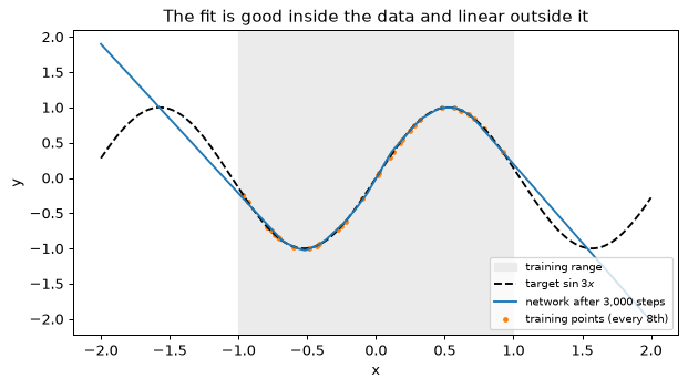
The training error falls by roughly three orders of magnitude. Inside the training range the network is indistinguishable from the sine. Outside it, the last linear piece of the ReLU network continues as a straight line, and the error on [1, 2] is of order one: a ReLU network is piecewise linear, so it extrapolates linearly, however well it interpolates. Nothing in the training loss can detect this, because no training point lies outside the range.
Step 7: what the initial scale does, over ten seeds
Section 6 argues that the initial scale of the weights sets the scale of the signal and of the gradients. A direct test replaces He initialisation with \mathcal{N}(0, 1) and with \mathcal{N}(0, 10^{-4}) (standard deviation 0.01). On a shallow network a single seed is misleading, because the initial loss depends strongly on the draw, so the experiment below uses ten initialisation seeds for each of the three schemes, the same data and the same 3,000 steps. It prints the median loss at steps 0, 100, 1,000 and 3,000 (and the range at step 0), and plots the median curve of each scheme on a logarithmic axis.
def init_scaled(scheme, seed):
    r = np.random.default_rng(100 + seed)
    if scheme == "He":
        s1, s2 = np.sqrt(2.0), np.sqrt(1 / 64)
    elif scheme == "N(0, 1)":
        s1 = s2 = 1.0
    else:                                        # "N(0, 1e-4)": standard deviation 0.01
        s1 = s2 = 0.01
    return {"W1": r.normal(0, s1, (1, 64)), "b1": np.zeros(64),
            "W2": r.normal(0, s2, (64, 1)), "b2": np.zeros(1)}


schemes = ["He", "N(0, 1)", "N(0, 1e-4)"]
curves = {}
for scheme in schemes:
    curves[scheme] = np.array([train(init_scaled(scheme, s), X, T, 3000, 0.05)
                               for s in range(10)])

for scheme in schemes:
    c = curves[scheme]
    print(f"{scheme:11s} step 0: median {np.median(c[:, 0]):.3g} "
          f"(range {c[:, 0].min():.3g} to {c[:, 0].max():.3g})")
    print(f"{'':11s} step 100: {np.median(c[:, 100]):.3g}   step 1000: "
          f"{np.median(c[:, 1000]):.3g}   final: {np.median(c[:, -1]):.2g}")
ratio = np.median(curves["N(0, 1e-4)"][:, -1]) / np.median(curves["He"][:, -1])
print(f"final loss, N(0, 1e-4) over He: {ratio:.0f} times")

plt.figure(figsize=(7, 4))
for scheme in schemes:
    plt.semilogy(np.median(curves[scheme], axis=0), label=scheme)
plt.xlabel("gradient-descent step")
plt.ylabel("training MSE (median of 10 seeds)")
plt.title("Initial scale and training speed")
plt.legend()
plt.tight_layout()
plt.show()
He          step 0: median 0.723 (range 0.185 to 2.02)
            step 100: 0.101   step 1000: 0.00501   final: 0.00035
N(0, 1)     step 0: median 7.87 (range 0.319 to 24.2)
            step 100: 0.0151   step 1000: 0.000582   final: 0.00023
N(0, 1e-4)  step 0: median 0.549 (range 0.549 to 0.55)
            step 100: 0.331   step 1000: 0.114   final: 0.009
final loss, N(0, 1e-4) over He: 26 times
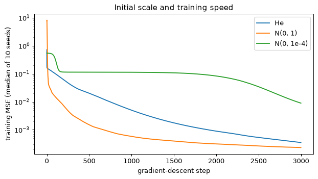
Read the table in three parts.
With \mathcal{N}(0, 1) the first-layer weights are somewhat smaller than He’s (standard deviation 1 against \sqrt 2) but the output weights are eight times larger than the variance 1/64 asks for, so the initial output is large: the median initial loss is about 8 and the range runs from 0.3 to 24, a factor of about seventy-five between seeds. At initialisation this zero-bias network is two random straight lines glued at a kink; a wild draw gives a wild line. The network is shallow, so gradient descent corrects it within a hundred steps, and the final loss is comparable to He’s. In a deep network the same excess would be multiplied at every layer, as the table of Section 6 shows.
With \mathcal{N}(0, 10^{-4}) the initial output is almost exactly zero, so the initial loss is the mean of t^2 for every seed. The gradient of each layer is proportional to the weights of the other, and both are tiny, so the gradient is tiny and the two layers must grow together before the fit can start: at step 1,000 the median loss is still 0.114, more than twenty times He’s, and after 3,000 steps it is about 26 times He’s. The network is in a flat region near the origin of weight space, not unable to learn, but it costs steps. With a deeper network the product of many tiny weights would make the region far flatter.
With He, the initial loss is moderate, there is no slow start, and the loss falls steadily.
What you should see
- The three well-behaved tensors of the gradient check agree with finite differences to roughly 10^{-8} or better; the bias of the first layer has one outlier whose smallest |z| is smaller than \epsilon_{\text{fd}}, and the outlier disappears at \epsilon_{\text{fd}} = 10^{-7}. A check is only as good as its \epsilon_{\text{fd}} and the smoothness of the function.
- The broken backward pass corrupts only \mathbf{W}^{(1)} and \mathbf{b}^{(1)}, the tensors below the missing gate: the check localises a bug to a layer.
- PyTorch agrees with the NumPy code to rounding error. Autograd computes the four equations of
Section 3; the stored weight layout,
(out, in), is the only difference. - The training error falls by three orders of magnitude, and the fit is good only inside the data’s range: outside it a ReLU network extrapolates linearly.
- The initial scale matters in both directions: too large gives a large and seed-dependent initial loss (0.3 to 24 over ten seeds), too small a slow start (a final loss 26 times He’s after the same 3,000 steps). Both are mild here because the network has one hidden layer, and both compound layer by layer in a deep one.
Try this
- Replace ReLU by \tanh in
forwardandbackward(\phi'(z) = 1 - \tanh^2 z, which is1 - H1 ** 2), rerun the gradient check and the training, and compare the final error with ReLU’s. The kink artefact of Step 3 should disappear. - Generalise
forwardandbackwardto L layers with loops over lists of weight matrices, gradient-check them, and repeat Step 7 with five hidden layers of 64 units. \mathcal{N}(0, 1) should now explode and \mathcal{N}(0, 10^{-4}) should stall. - Engineering variant: fit the neo-Hookean nominal stress P = 2c_1(\lambda - \lambda^{-2}) of Module 01, Section 12 (c_1 = 10 kPa, stretches \lambda from 0.6 to 1.0, 2% noise) with this network, and compare its prediction at \lambda = 0.5 with the one-parameter physical model’s. Which of the two extrapolates, and why?
- Switch to mini-batches of 32 and compare the loss curves with full-batch training at the same number of epochs.
Lab 2 — A scalar autodiff engine in about 100 lines
Goal. You build reverse-mode automatic differentiation from scratch: a Value class that
records the computational graph of Section 4 as the program runs, and a backward method
that sweeps the graph once and leaves \partial f/\partial v on every node. You check it by hand,
against finite differences and against PyTorch, and then use it, with no tensors at all, to train
a 337-parameter MLP on the two-moons problem. The engine works on one number at a time, so it is
slow by design; the last step measures how slow, and why that is what tensor frameworks exist to
fix. No download; the whole lab runs in under a minute, most of it in the training loop.
Step 1: a node that remembers how it was made
Reverse mode needs, for every intermediate result v, the list of values it was computed from (its parents) and the local partial derivative \partial v/\partial u for each parent u. The engine computes these local derivatives during the forward pass, when the operands are at hand, and stores them in the node. The backward sweep then needs no knowledge of what the operation was: it only multiplies and adds.
The class has four fields. data is the value, grad accumulates \partial f/\partial v for
the output f of the whole computation (the adjoint), _parents and _local are the two
tuples just described. __slots__ makes each node smaller and faster, which matters when a
single training step creates tens of thousands of them (Step 5 counts them). Each operator builds a new Value.
Subtraction is addition of a negation and negation is multiplication by the constant -1, and
division is multiplication by a power -1, so only five primitives need their own derivative:
+, \times, a constant power, and the functions below. Plain Python numbers are wrapped into
constant nodes by _wrap, which is also what makes 2 * x and 1 + x work through
__rmul__ and __radd__.
The derivatives are the ones of Section 4: for v = u + w both local derivatives are 1; for v = uw they are w and u; for v = u^k it is ku^{k-1}; for \exp, \log, \sin, \tanh and ReLU they are e^u, 1/u, \cos u, 1 - \tanh^2 u and \mathbb{1}[u > 0].
import math
import random
import time

import numpy as np
import matplotlib.pyplot as plt


class Value:
    """A scalar that records how it was computed."""
    __slots__ = ("data", "grad", "_parents", "_local")

    def __init__(self, data, parents=(), local=()):
        self.data = float(data)
        self.grad = 0.0                  # d(output)/d(this node), filled by backward()
        self._parents = parents          # the nodes this one was computed from
        self._local = local              # d(this node)/d(parent), one number per parent

    def __add__(self, other):
        other = _wrap(other)
        return Value(self.data + other.data, (self, other), (1.0, 1.0))

    def __mul__(self, other):
        other = _wrap(other)
        return Value(self.data * other.data, (self, other), (other.data, self.data))

    def __pow__(self, k):                # constant exponent only
        assert isinstance(k, (int, float))
        return Value(self.data ** k, (self,), (k * self.data ** (k - 1),))

    def __neg__(self):
        return self * -1

    def __sub__(self, other):
        return self + (-_wrap(other))

    def __rsub__(self, other):
        return _wrap(other) + (-self)

    def __truediv__(self, other):
        return self * _wrap(other) ** -1

    def __rtruediv__(self, other):
        return _wrap(other) * self ** -1

    __radd__ = __add__
    __rmul__ = __mul__


def _wrap(x):
    return x if isinstance(x, Value) else Value(x)


def exp(x):
    e = math.exp(x.data)
    return Value(e, (x,), (e,))


def log(x):
    return Value(math.log(x.data), (x,), (1.0 / x.data,))


def sin(x):
    return Value(math.sin(x.data), (x,), (math.cos(x.data),))


def tanh(x):
    t = math.tanh(x.data)
    return Value(t, (x,), (1.0 - t * t,))


def relu(x):
    return Value(max(x.data, 0.0), (x,), (1.0 if x.data > 0 else 0.0,))


a = Value(3.0)
b = a * a + 2 * a
print(f"b = a*a + 2*a at a = 3: data {b.data:.1f}, parents {len(b._parents)}, "
      f"local derivatives {b._local}")
b = a*a + 2*a at a = 3: data 15.0, parents 2, local derivatives (1.0, 1.0)
b is an addition node whose two parents are the product a \cdot a and the product 2 \cdot a;
nothing has been differentiated yet. The graph is the record of the computation, and the local
derivatives are the only calculus the engine will ever do.
Step 2: the backward sweep
Reverse mode is the chain rule applied once per edge, in the right order. Set \partial f/\partial f = 1 on the output. Then visit the nodes so that each node is visited only after every node that uses it, and for each parent u of the current node v add
The += is the whole treatment of fan-out: a variable used in three places receives three
contributions, and the multivariable chain rule says they add. (In b = a*a + 2*a the node a
is used three times and its gradient is a + a + 2 = 8.)
“Each node after all its users” is a reverse topological order, and the engine finds it with a depth-first traversal. The traversal below is iterative, with an explicit stack. A recursive one uses a Python stack frame per node on the current path, the loss of Step 5 is a running sum over the examples, and a longer sum or a deeper network would exceed Python’s default recursion limit of 1,000 frames. A node is pushed twice, once to be expanded and once, after its parents, to be emitted. Defining the method after the class and attaching it keeps the explanation of Step 1 separate from this one.
def backward(self):
    """Fill .grad on every node that self depends on. Returns the node count."""
    order, seen, stack = [], set(), [(self, False)]
    while stack:
        node, expanded = stack.pop()
        if expanded:
            order.append(node)           # all of its parents are already in `order`
            continue
        if id(node) in seen:
            continue
        seen.add(id(node))
        stack.append((node, True))
        for parent in node._parents:
            if id(parent) not in seen:
                stack.append((parent, False))
    self.grad = 1.0
    for node in reversed(order):         # users before the nodes they use
        for parent, local in zip(node._parents, node._local):
            parent.grad += node.grad * local
    return len(order)


Value.backward = backward

a = Value(3.0)
b = a * a + 2 * a
n_nodes = b.backward()
print(f"b = {b.data:.1f}, db/da = {a.grad:.1f} (analytic 2a + 2 = 8), nodes: {n_nodes}")
b = 15.0, db/da = 8.0 (analytic 2a + 2 = 8), nodes: 5
The engine proper (the Value class, the five functions and backward) is about 90 lines.
Everything else in the lab is using it.
Step 3: verify on a function with a known answer
Section 4 differentiates f(x_1, x_2) = \ln x_1 + x_1 x_2 - \sin x_2 by hand at (2, 5): \partial f/\partial x_1 = 1/x_1 + x_2 = 5.5 and \partial f/\partial x_2 = x_1 - \cos x_2 = 2 - \cos 5 \approx 1.7163. The next block computes it with the engine and with central differences on the same function written in plain floats, so that there are two independent references. The graph has nine nodes: two inputs, \ln x_1, x_1 x_2, their sum, \sin x_2, the constant -1 that subtraction creates, the negated sine, and the final sum.
x1, x2 = Value(2.0), Value(5.0)
f = log(x1) + x1 * x2 - sin(x2)
n_nodes = f.backward()
print(f"f = {f.data:.4f}   df/dx1 = {x1.grad:.4f}   df/dx2 = {x2.grad:.4f}   nodes: {n_nodes}")


def f_plain(u, v):
    return math.log(u) + u * v - math.sin(v)


eps = 1e-6
fd1 = (f_plain(2 + eps, 5) - f_plain(2 - eps, 5)) / (2 * eps)
fd2 = (f_plain(2, 5 + eps) - f_plain(2, 5 - eps)) / (2 * eps)
print(f"finite differences: {fd1:.4f} and {fd2:.4f}")
print(f"largest difference from the engine: {max(abs(fd1 - x1.grad), abs(fd2 - x2.grad)):.1e}")
f = 11.6521   df/dx1 = 5.5000   df/dx2 = 1.7163   nodes: 9
finite differences: 5.5000 and 1.7163
largest difference from the engine: 4.5e-10
The cost of the engine’s answer is one forward evaluation and one sweep for both partial derivatives; finite differences needed four extra function evaluations for two inputs, and would need 2n for n inputs. That asymmetry is why reverse mode is used for networks with millions of parameters.
Step 4: neurons, layers and an MLP
An MLP made of Values is a few lines. A Neuron holds one weight Value per input and a bias,
computes \sum_j w_j x_j + b and optionally applies ReLU. Weights are drawn from \mathcal{N}(0, 2/n_{\text{in}}),
He initialisation as in Section 6, and biases start at zero. random.gauss is used instead
of NumPy so that the engine depends on nothing but the standard library. MLP(2, [16, 16, 1]) is
the 2 \to 16 \to 16 \to 1 network with ReLU in the two hidden layers and a linear output (the
output is a logit), so its parameter count is (2 \cdot 16 + 16) + (16 \cdot 16 + 16) + (16 + 1).
class Neuron:
    def __init__(self, n_in, nonlinear):
        std = math.sqrt(2.0 / n_in)
        self.w = [Value(random.gauss(0.0, std)) for _ in range(n_in)]
        self.b = Value(0.0)
        self.nonlinear = nonlinear

    def __call__(self, x):
        z = sum((w * xi for w, xi in zip(self.w, x)), self.b)
        return relu(z) if self.nonlinear else z

    def parameters(self):
        return self.w + [self.b]


class Layer:
    def __init__(self, n_in, n_out, nonlinear):
        self.neurons = [Neuron(n_in, nonlinear) for _ in range(n_out)]

    def __call__(self, x):
        return [neuron(x) for neuron in self.neurons]

    def parameters(self):
        return [p for neuron in self.neurons for p in neuron.parameters()]


class MLP:
    def __init__(self, n_in, widths):
        sizes = [n_in] + widths
        self.layers = [Layer(sizes[i], sizes[i + 1], nonlinear=(i < len(widths) - 1))
                       for i in range(len(widths))]

    def __call__(self, x):
        for layer in self.layers:
            x = layer(x)
        return x

    def parameters(self):
        return [p for layer in self.layers for p in layer.parameters()]


random.seed(0)
model = MLP(2, [16, 16, 1])
params = model.parameters()
print("parameters:", len(params))
parameters: 337
Step 5: the loss, and training
The task is make_moons: two interleaved half-circles, labels 0 and 1, 100 training points. The loss is the mean binary cross-entropy computed from the logit z in the stable form of Section 12,
which never exponentiates a large positive number. The engine has no abs, but
|z| = \max(z, 0) + \max(-z, 0) is built from two ReLUs, so the loss uses only primitives that
already exist. (At this size a naive sigmoid would also work; the stable form is the habit to
build, and it costs nothing.)
Training is full-batch gradient descent with \eta = 1.0. Two details are easy to get wrong.
Gradients accumulate with +=, so they must be zeroed on every parameter before each backward
pass; and the parameters are Values whose data is changed in place, while every other node is
rebuilt on each step. The loop evaluates the loss before updating, so the number printed at step
k is the loss of the parameters after k updates; at step 100 only the evaluation and the
backward pass are done, which leaves the gradient at the final parameters for the PyTorch
comparison of Step 7. The graph size (nodes, the number of nodes in the graph of one
loss evaluation) is printed too.
from sklearn.datasets import make_moons

X_train, y_train = make_moons(n_samples=100, noise=0.1, random_state=0)
X_test, y_test = make_moons(n_samples=500, noise=0.1, random_state=1)


def bce_with_logits(z, y):
    """Stable binary cross-entropy of logit z (a Value) and label y in {0, 1}."""
    abs_z = relu(z) + relu(-z)
    return relu(z) - z * y + log(1.0 + exp(-abs_z))


def loss_and_accuracy(model, X, y):
    total, correct = Value(0.0), 0
    for xi, yi in zip(X, y):
        z = model([Value(xi[0]), Value(xi[1])])[0]   # inputs wrapped once per example
        total = total + bce_with_logits(z, float(yi))
        correct += int((z.data > 0) == (yi == 1))
    return total * (1.0 / len(X)), correct / len(X)


eta = 1.0
for step in range(101):
    for p in params:
        p.grad = 0.0                     # gradients accumulate, so zero them first
    loss, acc = loss_and_accuracy(model, X_train, y_train)
    n_nodes = loss.backward()
    if step % 20 == 0:
        print(f"step {step:3d}  loss {loss.data:.3f}  train accuracy {acc:.2f}  "
              f"nodes {n_nodes:,}")
    if step < 100:
        for p in params:
            p.data -= eta * p.grad
final_loss = loss.data
step   0  loss 1.065  train accuracy 0.29  nodes 66,440
step  20  loss 0.198  train accuracy 0.92  nodes 66,440
step  40  loss 0.197  train accuracy 0.96  nodes 66,440
step  60  loss 0.131  train accuracy 0.97  nodes 66,440
step  80  loss 0.074  train accuracy 0.98  nodes 66,440
step 100  loss 0.035  train accuracy 0.99  nodes 66,440
The initial loss is above \ln 2 = 0.693, the loss of a classifier that outputs probability 1/2 everywhere. The cause is the output neuron: it is initialised like a hidden one, with variance 2/16, so its logits start with a spread of order one, and a confident wrong logit is punished harder than a hesitant one. Section 14’s initial-loss check would flag this; the remedy is a smaller output initialisation. It is left as it is because the network recovers within twenty steps, as the table shows. The graph holds 66,440 nodes for 100 examples and 337 parameters: it is the tape of Section 4, and its size is the memory price of reverse mode.
Step 6: test accuracy and the decision boundary
The test accuracy needs no gradients, so it should not build a graph. The next block extracts the trained weights into NumPy arrays and runs a plain float forward pass, which is also how a deployed model works. The decision boundary is the zero contour of the logit on a 100 \times 100 grid.
def extract_arrays(model):
    """Weights as (n_in, n_out) arrays, biases as (n_out,) arrays, per layer."""
    arrays = []
    for layer in model.layers:
        W = np.array([[w.data for w in neuron.w] for neuron in layer.neurons]).T
        b = np.array([neuron.b.data for neuron in layer.neurons])
        arrays.append((W, b))
    return arrays


def float_logits(arrays, X):
    H = X
    for i, (W, b) in enumerate(arrays):
        H = H @ W + b
        if i < len(arrays) - 1:
            H = np.maximum(H, 0)
    return H[:, 0]


arrays = extract_arrays(model)
test_accuracy = np.mean((float_logits(arrays, X_test) > 0) == (y_test == 1))
print(f"test accuracy on 500 points: {test_accuracy:.3f}")

gx, gy = np.meshgrid(np.linspace(-1.6, 2.6, 100), np.linspace(-1.1, 1.6, 100))
grid_logits = float_logits(arrays, np.c_[gx.ravel(), gy.ravel()]).reshape(gx.shape)
plt.figure(figsize=(6, 4.5))
plt.contourf(gx, gy, grid_logits > 0, levels=[-0.5, 0.5, 1.5], colors=["#cfe3f5", "#f8d9c4"])
plt.scatter(*X_train[y_train == 0].T, s=14, color="C0", label="class 0 (training)")
plt.scatter(*X_train[y_train == 1].T, s=14, color="C1", label="class 1 (training)")
plt.xlabel("$x_1$")
plt.ylabel("$x_2$")
plt.title("Moons: decision regions of the scalar-engine MLP")
plt.legend(loc="upper right", fontsize=8)
plt.tight_layout()
plt.show()
test accuracy on 500 points: 0.992
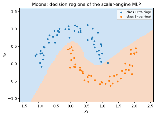
Step 7: PyTorch as a referee
The engine’s weights are copied into float64 tensors and the same loss is computed with
F.binary_cross_entropy_with_logits on the same training points. backward() then gives
PyTorch’s gradients, which are compared with the engine’s, parameter by parameter. The engine
stores a neuron per object, PyTorch a matrix per layer, so the engine’s flat parameter list is
matched to the arrays through the same ordering (weights of neuron 0, its bias, weights of
neuron 1, ...).
import torch
import torch.nn.functional as F

tensors = [(torch.tensor(W, dtype=torch.float64, requires_grad=True),
            torch.tensor(b, dtype=torch.float64, requires_grad=True)) for W, b in arrays]


def torch_logits(tensors, X):
    H = torch.tensor(X, dtype=torch.float64)
    for i, (W, b) in enumerate(tensors):
        H = H @ W + b
        if i < len(tensors) - 1:
            H = torch.relu(H)
    return H[:, 0]


loss_torch = F.binary_cross_entropy_with_logits(
    torch_logits(tensors, X_train), torch.tensor(y_train, dtype=torch.float64))
loss_torch.backward()

engine_grads = []        # in the engine's parameter order: per neuron, weights then bias
for layer, (W, b) in zip(model.layers, tensors):
    for j, neuron in enumerate(layer.neurons):
        engine_grads += [(w.grad, W.grad[i, j].item()) for i, w in enumerate(neuron.w)]
        engine_grads.append((neuron.b.grad, b.grad[j].item()))
gap = max(abs(a - t) for a, t in engine_grads)
print(f"loss: engine {final_loss:.10f}   PyTorch {loss_torch.item():.10f}")
print(f"largest gradient difference over {len(engine_grads)} parameters: {gap:.1e}")
loss: engine 0.0347593932   PyTorch 0.0347593932
largest gradient difference over 337 parameters: 3.5e-17
The two frameworks give the same loss and the same 337 gradients to rounding error. The engine is a toy, but it is not a different kind of object from autograd: PyTorch records a graph of tensor operations, each with a function that maps an incoming adjoint to adjoints of its inputs (a vector-Jacobian product), and sweeps it in reverse.
Step 8: what the tensor version buys
One forward and backward pass of the engine on the 100 training points is timed against the same computation in PyTorch, after a warm-up call, averaged over 200 repetitions. Both do identical arithmetic. The difference is entirely overhead: the engine creates 66,440 Python objects and runs a Python loop over every edge, where PyTorch issues about ten tensor operations that run in compiled code.
def engine_step():
    for p in params:
        p.grad = 0.0
    loss, _ = loss_and_accuracy(model, X_train, y_train)
    loss.backward()


def torch_step():
    for W, b in tensors:
        W.grad = None
        b.grad = None
    F.binary_cross_entropy_with_logits(
        torch_logits(tensors, X_train),
        torch.tensor(y_train, dtype=torch.float64)).backward()


start = time.perf_counter()
engine_step()
engine_seconds = time.perf_counter() - start

torch_step()                              # warm-up
start = time.perf_counter()
for _ in range(200):
    torch_step()
torch_seconds = (time.perf_counter() - start) / 200
ratio = engine_seconds / torch_seconds
print(f"engine over 0.05 s per step: {engine_seconds > 0.05}   "
      f"PyTorch under 1 ms: {torch_seconds < 1e-3}")   # exact times vary by machine
print(f"ratio, to the nearest power of ten: {10 ** round(math.log10(ratio)):,}")
engine over 0.05 s per step: True   PyTorch under 1 ms: True
ratio, to the nearest power of ten: 1,000
The exact times vary from run to run and from machine to machine (the engine takes a few tenths of a second per step on a laptop), so the block prints two thresholds and the ratio to the nearest power of ten. PyTorch’s per-operation overhead means that its advantage grows with the tensor sizes: on a larger matrix product the compiled code does thousands of multiplications per call, where the engine’s loop would do them one at a time.
What you should see
- Reverse mode takes a few dozen lines once each primitive knows its local derivative. The
+=in the backward sweep is what handles a variable used more than once. - The engine reproduces the hand-computed gradients of the Section 4 example, agrees with finite differences, and gives the same 337 gradients as PyTorch to rounding error.
- Memory and time grow with the number of graph nodes: 66,440 for 100 examples through 337 parameters. The tape is the price of reverse mode.
- The initial loss is above \ln 2 because the output neuron has the He scale; the initial-loss check of Section 14 would catch it, and a smaller output initialisation fixes it.
- With \eta = 1.0 the MLP fits the moons in 100 steps. The learning rate matters even for a toy (Section 9).
Try this
- Add a softplus primitive, \ln(1 + e^x), and a
tanhoption for the hidden layers, and compare the training curves with ReLU’s. - Add forward mode: give
Valueatangentfield propagated by every operation, and compute \partial f/\partial x_1 of the Section 4 example in one forward pass. Count how many passes the gradient with respect to both inputs needs. - Support a
Valueexponent inx ** yand check the gradient with respect to both arguments by finite differences. Which argument’s derivative has a domain restriction? - Write a micro tensor version in which
datais a NumPy array and each operation stores a VJP function instead of scalar local derivatives, and time it against the scalar engine. - Train with \eta = 0.5 for 50 steps and then \eta = 0.1, and compare the accuracy at step 100 with the run above.
Lab 3 — Optimisers, schedules and the range test
Goal. You find learning rates with a range test instead of guessing them, then run SGD, momentum, Nesterov momentum, Adam and AdamW on the same network and data from the same initialisation, and read what the differences are and are not. A second experiment measures what a learning-rate schedule does to the noise floor of a noisy regression, and a last one verifies the sign-descent behaviour of Adam’s first step. The lab uses the digits data that ships with scikit-learn and a synthetic regression, so nothing is downloaded, and it runs in under half a minute of CPU time. Its network, a 64 \to 128 \to 128 \to 10 ReLU MLP with 26,122 parameters, is the digits network of Section 2 and the one Lab 4 trains in full.
Step 1: the data
load_digits holds 1,797 images of 8 by 8 pixels with 10 classes. The split is 60/20/20,
stratified so that every class keeps its share, which gives 1,078 training, 359 validation and
360 test images. Standardisation uses the training statistics only, as Module 01, Section 10
requires: a statistic computed on the validation or test images would leak them into training. A
few pixels are constant (always zero) in the training set; their standard deviation is replaced by 1
so the division is defined and the standardised column stays zero. The test set is not touched in
this lab.
import time

import numpy as np
import torch
import torch.nn as nn
import torch.nn.functional as F
import matplotlib.pyplot as plt
from sklearn.datasets import load_digits
from sklearn.model_selection import train_test_split

digits = load_digits()
X_all, y_all = digits.data.astype(np.float32), digits.target
X_tr, X_rest, y_tr, y_rest = train_test_split(
    X_all, y_all, test_size=0.4, stratify=y_all, random_state=0)
X_va, X_te, y_va, y_te = train_test_split(
    X_rest, y_rest, test_size=0.5, stratify=y_rest, random_state=0)

mean = X_tr.mean(axis=0)
std = X_tr.std(axis=0)
std[std == 0] = 1.0                       # constant pixels: leave them at zero
as_tensor = lambda a: torch.tensor((a - mean) / std)

Xtr, Xva = as_tensor(X_tr), as_tensor(X_va)
ytr, yva = torch.tensor(y_tr), torch.tensor(y_va)
print("split sizes:", len(X_tr), len(X_va), len(X_te))
print("constant pixels in the training set:", int((X_tr.std(axis=0) == 0).sum()))
split sizes: 1078 359 360
constant pixels in the training set: 4
Step 2: the model and the evaluation function
make(seed) builds the network under torch.manual_seed(seed), so the same seed gives the same
initial weights (PyTorch’s default initialisation, which for nn.Linear is a uniform
distribution whose variance is 1/(3 n_{\text{in}}); Section 6 discusses how it
compares with He’s). evaluate returns the loss and the accuracy. It calls model.eval() and
runs under torch.no_grad(), the two habits of Section 13: the model has no dropout or
batch norm yet, so eval() changes nothing here, but the habit costs nothing and the day it
matters it matters a great deal.
def make(seed):
    torch.manual_seed(seed)
    return nn.Sequential(nn.Linear(64, 128), nn.ReLU(),
                         nn.Linear(128, 128), nn.ReLU(),
                         nn.Linear(128, 10))


def evaluate(model, X, y):
    model.eval()
    with torch.no_grad():
        logits = model(X)
        return F.cross_entropy(logits, y).item(), (logits.argmax(1) == y).float().mean().item()


model = make(0)
print("parameters:", sum(p.numel() for p in model.parameters()))
loss0, acc0 = evaluate(model, Xtr, ytr)
print(f"untrained: training loss {loss0:.3f} (ln 10 = {np.log(10):.3f}), accuracy {acc0:.3f}")
parameters: 26122
untrained: training loss 2.309 (ln 10 = 2.303), accuracy 0.106
An untrained 10-class classifier should have a loss near \ln 10, the loss of the uniform prediction (Section 14, the initial-loss check). That is what the run shows to the precision that a random initialisation allows.
Step 3: the range test, written out
The learning-rate range test of Section 9 trains for a short run while the learning rate grows geometrically, and records the loss. At a very small rate nothing happens; at a good rate the loss falls fast; past the largest stable rate it rises and the run diverges. The block below runs 200 steps with \eta growing from 10^{-5} to 10, so that every step multiplies it by the same factor (10^{6})^{1/199}, with mini-batches of 64 cycled through the training set. The raw mini-batch loss is noisy, so what is recorded is its exponential moving average with factor 0.9, corrected for the bias that starts it at zero (the same correction as Adam’s). The test stops when the smoothed loss exceeds four times its minimum, and returns three read-outs: the rate at the steepest fall of the smoothed loss against \log \eta, the rate at its minimum, and the rate at which the run was stopped. The usual choice is a rate a factor of several below the minimum, near the steepest fall.
def range_test(optimiser_factory, lr_min=1e-5, lr_max=10.0, steps=200, batch=64, seed=0):
    model = make(seed)
    optimiser = optimiser_factory(model.parameters(), lr_min)
    gamma = (lr_max / lr_min) ** (1 / (steps - 1))        # constant factor per step
    order = torch.cat([torch.randperm(len(Xtr), generator=torch.Generator().manual_seed(k))
                       for k in range(steps * batch // len(Xtr) + 1)])
    lrs, smooth, running, best = [], [], 0.0, float("inf")
    for step in range(steps):
        lr = lr_min * gamma ** step
        for group in optimiser.param_groups:
            group["lr"] = lr
        idx = order[step * batch:(step + 1) * batch]
        model.train()
        loss = F.cross_entropy(model(Xtr[idx]), ytr[idx])
        optimiser.zero_grad()
        loss.backward()
        optimiser.step()
        running = 0.9 * running + 0.1 * loss.item()
        value = running / (1 - 0.9 ** (step + 1))           # bias-corrected average
        lrs.append(lr)
        smooth.append(value)
        best = min(best, value)
        if not np.isfinite(value) or value > 4 * best:       # diverged: stop
            break
    lrs, smooth = np.array(lrs), np.array(smooth)
    slope = np.gradient(smooth, np.log10(lrs))               # change per decade of lr
    return {"lrs": lrs, "smooth": smooth, "steps": len(lrs),
            "steepest": lrs[np.argmin(slope)], "minimum": lrs[np.argmin(smooth)],
            "min_loss": smooth.min(), "stopped": lrs[-1]}


sgd_factory = lambda params, lr: torch.optim.SGD(params, lr=lr, momentum=0.9)
adam_factory = lambda params, lr: torch.optim.Adam(params, lr=lr)
tests = {"SGD + momentum 0.9": range_test(sgd_factory), "Adam": range_test(adam_factory)}
for name, r in tests.items():
    print(f"{name:20s} steepest fall at lr {r['steepest']:.2g}; minimum {r['min_loss']:.3f} "
          f"at lr {r['minimum']:.2g}; stopped at lr {r['stopped']:.2g} (step {r['steps']})")
SGD + momentum 0.9   steepest fall at lr 0.048; minimum 0.310 at lr 0.44; stopped at lr 0.58 (step 159)
Adam                 steepest fall at lr 0.0024; minimum 0.249 at lr 0.017; stopped at lr 0.089 (step 132)
Step 4: reading the two curves
The plot puts the smoothed loss against the learning rate on a logarithmic axis, for both optimisers. Vertical lines mark the steepest fall. Read it from left to right: a flat stretch where the rate is too small to move the loss in 200 steps, a descent, a minimum, and a rise to the point where the run was stopped.
fig, ax = plt.subplots(figsize=(7, 4))
for (name, r), colour in zip(tests.items(), ["C0", "C1"]):
    ax.plot(r["lrs"], r["smooth"], color=colour, label=name)
    ax.axvline(r["steepest"], color=colour, linestyle=":", label=f"{name}: steepest fall")
ax.set_xscale("log")
ax.set_xlabel("learning rate (grows by a constant factor per step)")
ax.set_ylabel("smoothed training loss")
ax.set_title("Learning-rate range test on the digits MLP")
ax.legend(fontsize=8)
plt.tight_layout()
plt.show()
The two optimisers do not share a scale. Adam’s steepest fall (0.0024) and its minimum (0.017) lie 20 and 26 times below those of SGD with momentum (0.048 and 0.44), and it diverges earlier, at 0.089 against 0.58. This is the same fact as Adam’s normalisation: its step is about \eta per parameter, whatever the gradient’s size, where SGD’s step is \eta times a gradient that is small for most parameters (Section 8). It is also why a learning rate found for one optimiser is useless for another.
Step 5: the shoot-out
Six optimiser settings, trained for 20 epochs from the same initial weights (seed 0) and with
the same order of mini-batches of 64, so that the only difference is the update rule. After every
epoch the loss on the whole training set is recorded (in eval() mode, without gradients), which is
a cleaner measure than the loss of the last mini-batch. The table reports the first epoch whose
full training loss is below 0.1, the final training loss, and the validation loss and accuracy.
The settings are SGD at \eta = 0.05 and at \eta = 0.5, momentum 0.9 at \eta = 0.05, Nesterov momentum 0.9 at \eta = 0.05, Adam at 2 \times 10^{-3} (near the range test’s steepest fall), and AdamW at the same rate with weight decay 10^{-2}.
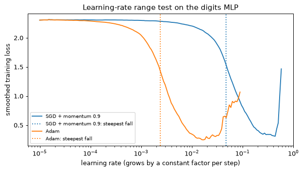
def train_run(optimiser_factory, epochs=20, batch=64, seed=0):
    model = make(seed)
    optimiser = optimiser_factory(model.parameters())
    shuffler = torch.Generator().manual_seed(123)         # same batch order for every run
    history = [evaluate(model, Xtr, ytr)[0]]
    for epoch in range(epochs):
        model.train()
        order = torch.randperm(len(Xtr), generator=shuffler)
        for i in range(0, len(Xtr), batch):
            idx = order[i:i + batch]
            loss = F.cross_entropy(model(Xtr[idx]), ytr[idx])
            optimiser.zero_grad()
            loss.backward()
            optimiser.step()
        history.append(evaluate(model, Xtr, ytr)[0])
    return model, history


configs = {
    "SGD 0.05": lambda ps: torch.optim.SGD(ps, lr=0.05),
    "SGD 0.5": lambda ps: torch.optim.SGD(ps, lr=0.5),
    "momentum 0.9, 0.05": lambda ps: torch.optim.SGD(ps, lr=0.05, momentum=0.9),
    "Nesterov 0.9, 0.05": lambda ps: torch.optim.SGD(ps, lr=0.05, momentum=0.9, nesterov=True),
    "Adam 2e-3": lambda ps: torch.optim.Adam(ps, lr=2e-3),
    "AdamW 2e-3, wd 1e-2": lambda ps: torch.optim.AdamW(ps, lr=2e-3, weight_decay=1e-2),
}
histories = {}
print(f"{'optimiser':22s} {'first epoch <0.1':>16s} {'train loss':>11s} "
      f"{'val loss':>9s} {'val acc':>8s}")
for name, factory in configs.items():
    model, history = train_run(factory)
    histories[name] = history
    below = [e for e, v in enumerate(history) if v < 0.1]
    first = str(below[0]) if below else "never"
    val_loss, val_acc = evaluate(model, Xva, yva)
    print(f"{name:22s} {first:>16s} {history[-1]:11.4f} {val_loss:9.3f} {val_acc:8.3f}")
optimiser              first epoch <0.1  train loss  val loss  val acc
SGD 0.05                          never      0.1289     0.212    0.933
SGD 0.5                               3      0.0027     0.093    0.975
momentum 0.9, 0.05                    4      0.0024     0.132    0.972
Nesterov 0.9, 0.05                    3      0.0025     0.103    0.975
Adam 2e-3                             4      0.0018     0.125    0.967
AdamW 2e-3, wd 1e-2                   4      0.0019     0.124    0.967
plt.figure(figsize=(7, 4))
for name, history in histories.items():
    plt.semilogy(history, marker="o", markersize=3, label=name)
plt.axhline(0.1, color="0.6", linestyle=":")
plt.xlabel("epoch (17 steps each)")
plt.ylabel("training loss on the whole training set")
plt.title("Six optimisers, same network, same start, same batches")
plt.legend(fontsize=8)
plt.tight_layout()
plt.show()
Four observations. First, plain SGD at \eta = 0.05 is slow, and it is slow in a specific way: its loss is still falling when training stops (0.129 after 20 epochs, a level the other settings passed in epoch 3 or 4), and its validation accuracy, 93.3%, is that of an unfinished run. Raising its rate to 0.5 fixes that, and on this problem 0.5 is stable. Second, momentum 0.9 at \eta = 0.05 behaves like plain SGD at 0.5, which is the effective learning rate \eta/(1 - \mu) of Section 7: with a steady gradient the velocity grows to 1/(1-\mu) = 10 times the gradient. The two curves are close but not identical, because the steady-gradient picture holds only where the gradient changes slowly. Third, Nesterov’s variant is almost indistinguishable from the classical one here; its advantage is a property of the analysis of smooth convex problems, not a visible effect on a problem this easy. Fourth, Adam is not faster than well-tuned SGD in reaching a training loss of 0.1 (epoch 4, against 3 for SGD at 0.5 and for Nesterov momentum), although it reaches the lowest final training loss, 0.0018; AdamW, with a decay of 10^{-2} that is small on this scale, differs from Adam only in the last digits. The five settings that train end with validation accuracies between 96.7% and 97.5%, a spread of 0.8 points. The binomial standard error of an accuracy near 97% on 359 images is \sqrt{0.97 \cdot 0.03 / 359} \approx 0.009, about one point, so the ranking among them is not established by this experiment. On an easy problem the choice of optimiser changes the speed, not the destination. (The validation loss, which is lower for SGD at 0.5 than for Adam, is a different matter: a network that has driven its training loss to 0.002 is confident, and its confidence is penalised on the images it gets wrong.)
Step 6: schedules and the noise floor of SGD
Section 9 argues that with a constant rate, SGD does not converge to the minimum but to a noise floor whose excess loss is proportional to \eta, and that a decaying schedule removes the excess. This step measures it. The data are a noisy regression, y = \sin 3x + 0.1\,\xi with \xi \sim \mathcal{N}(0, 1), 4,096 training and 2,048 validation points, so that even the true function has a validation MSE equal to the noise variance, about 0.01: that number, computed in the first print, is the best that any model can reach, and the excess over it is what the schedule controls. A 1 \to 64 \to 64 \to 1 ReLU network is trained with SGD, momentum 0.9, peak \eta = 0.05, batches of 32 and 20 epochs (2,560 steps) under three schedules: constant; step decay (\times 0.1 at 50% and \times 0.01 at 75% of the steps); and 5% linear warmup followed by cosine decay to zero. The initial weights and the batch order are the same for all three.
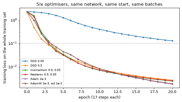
torch.manual_seed(0)
x_tr = torch.rand(4096, 1) * 2 - 1
y_tr_reg = torch.sin(3 * x_tr) + 0.1 * torch.randn(4096, 1)
x_va = torch.rand(2048, 1) * 2 - 1
y_va_reg = torch.sin(3 * x_va) + 0.1 * torch.randn(2048, 1)
noise_floor = F.mse_loss(torch.sin(3 * x_va), y_va_reg).item()
print(f"noise floor: validation MSE of the true function = {noise_floor:.4f}")


def make_regressor(seed=0):
    torch.manual_seed(seed)
    return nn.Sequential(nn.Linear(1, 64), nn.ReLU(), nn.Linear(64, 64), nn.ReLU(),
                         nn.Linear(64, 1))


def lr_factor(kind, step, total):
    """Multiplier on the peak learning rate at a given step."""
    if kind == "constant":
        return 1.0
    if kind == "step":
        return 1.0 if step < 0.5 * total else (0.1 if step < 0.75 * total else 0.01)
    warm = int(0.05 * total)                               # cosine with 5% linear warmup
    if step < warm:
        return (step + 1) / warm
    return 0.5 * (1 + np.cos(np.pi * (step - warm) / (total - warm)))


def run_schedule(kind, peak=0.05, epochs=20, batch=32, seed=0):
    model = make_regressor(seed)
    optimiser = torch.optim.SGD(model.parameters(), lr=peak, momentum=0.9)
    shuffler = torch.Generator().manual_seed(7)
    total, step, val_curve, lr_curve = epochs * (4096 // batch), 0, [], []
    for epoch in range(epochs):
        model.train()
        order = torch.randperm(4096, generator=shuffler)
        for i in range(0, 4096, batch):
            for group in optimiser.param_groups:
                group["lr"] = peak * lr_factor(kind, step, total)
            idx = order[i:i + batch]
            loss = F.mse_loss(model(x_tr[idx]), y_tr_reg[idx])
            optimiser.zero_grad()
            loss.backward()
            optimiser.step()
            lr_curve.append(optimiser.param_groups[0]["lr"])
            step += 1
        model.eval()
        with torch.no_grad():
            val_curve.append(F.mse_loss(model(x_va), y_va_reg).item())
    return np.array(val_curve), np.array(lr_curve)


results = {kind: run_schedule(kind) for kind in ["constant", "step", "cosine"]}
for kind, (val_curve, _) in results.items():
    final = val_curve[-1]
    print(f"{kind:9s} final validation MSE {final:.5f} (excess over the floor "
          f"{100 * (final - noise_floor) / noise_floor:5.1f}%), "
          f"std of the last five epochs {val_curve[-5:].std():.5f}")
noise floor: validation MSE of the true function = 0.0104
constant  final validation MSE 0.01305 (excess over the floor  25.7%), std of the last five epochs 0.00074
step      final validation MSE 0.01041 (excess over the floor   0.2%), std of the last five epochs 0.00002
cosine    final validation MSE 0.01043 (excess over the floor   0.4%), std of the last five epochs 0.00011
fig, (ax_lr, ax_val) = plt.subplots(1, 2, figsize=(10, 3.8))
for kind, (val_curve, lr_curve) in results.items():
    ax_lr.plot(lr_curve, label=kind)
    ax_val.plot(np.arange(1, 21), val_curve - noise_floor, marker="o", markersize=3, label=kind)
ax_lr.set_xlabel("step")
ax_lr.set_ylabel("learning rate")
ax_lr.set_title("The three schedules")
ax_lr.legend(fontsize=8)
ax_val.set_yscale("symlog", linthresh=1e-4)
ax_val.set_xlabel("epoch")
ax_val.set_ylabel("validation MSE minus the noise floor")
ax_val.set_title("Excess validation loss under each schedule")
ax_val.legend(fontsize=8)
plt.tight_layout()
plt.show()
The constant rate ends 26% above the floor, and its last five epochs vary with a standard deviation of about 7 \times 10^{-4}; the two decaying schedules end within half a per cent of the floor, and their last epochs barely move. The excess of the constant schedule is the noise floor of SGD: the iterate keeps being kicked by the gradient noise of mini-batches, and the size of the kicks is set by \eta. Decaying the rate shrinks the kicks. Note also that the two decaying schedules are indistinguishable at this scale; what matters is that the rate reaches a small value, not the shape of the path. The comparison is one run per schedule, and the size of the constant schedule’s excess is the value of one last point of a jittering curve, not an average: the last Try-this item separates the trend from the chance.
Step 7: Adam’s first step is sign descent
At the first step t = 1 the moment estimates are m = (1 - \beta_1) g and v = (1 - \beta_2) g^2, and after the bias correction of Section 8 \hat m = g and \hat v = g^2, so the update is \eta\, g / (|g| + \epsilon) \approx \eta\,\mathrm{sign}(g): every parameter with a non-negligible gradient moves by almost exactly \eta, whether its gradient is 10^{-7} or 10^{-2}. The block checks it on the digits network: one Adam step with \eta = 10^{-3} on the first batch of 64 training images from a fresh model. It counts the parameters whose gradient is exactly zero, reports the range of the other gradient magnitudes, and the fraction of those parameters that moved by more than 0.99\eta.
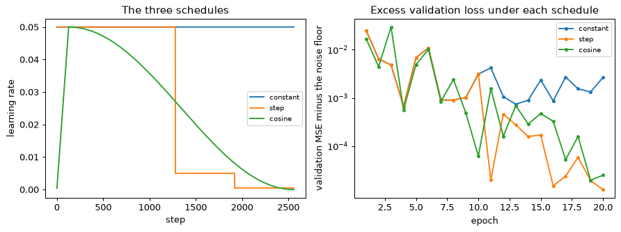
model = make(0)
optimiser = torch.optim.Adam(model.parameters(), lr=1e-3)
idx = torch.arange(64)
F.cross_entropy(model(Xtr[idx]), ytr[idx]).backward()
before = torch.cat([p.detach().flatten().clone() for p in model.parameters()])
grads = torch.cat([p.grad.flatten() for p in model.parameters()])
optimiser.step()
after = torch.cat([p.detach().flatten() for p in model.parameters()])

nonzero = grads != 0
moved = (after - before).abs()[nonzero]
print(f"parameters with an exactly zero gradient: {int((~nonzero).sum())} of {grads.numel()}")
print(f"non-zero gradient magnitudes: {grads[nonzero].abs().min():.1e} "
      f"to {grads[nonzero].abs().max():.1e}")
print(f"fraction of those that moved by more than 0.99 * lr: "
      f"{(moved > 0.99e-3).float().mean():.4f}")
parameters with an exactly zero gradient: 615 of 26122
non-zero gradient magnitudes: 1.8e-07 to 6.4e-02
fraction of those that moved by more than 0.99 * lr: 0.9996
The step sizes of the parameters differ by almost nothing, although the gradients differ over more than five orders of magnitude. This is Adam’s strength and its hazard. It is a strength because parameters with tiny gradients (a rarely used embedding, a layer far from the loss) still move at a useful rate. It is a hazard because a parameter whose gradient is pure noise moves just as far: this is the reason Adam needs a warmup when \beta_2 is close to 1 and the second-moment estimate is poor in the first steps (Section 9). The zero-gradient parameters do not move, because 0/(0 + \epsilon) = 0. Of the 615, 512 are the first-layer weights of the four constant pixels (4 \times 128); the other 103 are second-layer weights for which no image of the batch has both the input unit and the output unit active, so the product h_i \delta_j of Section 3 is zero on every example.
What you should see
- The range test finds the right decade in seconds. Adam’s usable range sits well below that of SGD with momentum: its steepest fall and its minimum are 20 and 26 times lower, and it diverges at a rate 6.5 times lower.
- Momentum 0.9 at \eta = 0.05 behaves like plain SGD at \eta = 0.5: the effective rate is \eta/(1 - \mu).
- Adam is not faster than well-tuned SGD with momentum on this easy problem, and the five settings that train end within 0.8 points of one another on validation accuracy, inside one standard error.
- A constant learning rate ends 26% above the noise floor (in this run) and jitters from epoch to epoch; both decaying schedules end within half a per cent of the floor.
- Adam’s first step moves almost every parameter by \eta, whatever the size of its gradient: sign descent.
Try this
- Add RMSprop and Adagrad (
torch.optim) to the shoot-out, with rates from your own range tests, and place them in the table. - Repeat the shoot-out with six hidden layers of 64 units and find where plain SGD stops working.
- Run AdamW at \eta = 3 \times 10^{-2} (above the range test’s minimum) with and without a 5% warmup, and plot the first 100 steps of each.
- Repeat Step 6 with three seeds at \eta = 0.02 and \eta = 0.05 and average the final MSE of the constant schedule, to separate the trend (excess proportional to \eta) from the randomness of the last point.
Lab 4 — Digits, honestly: a complete PyTorch training run
Goal. You train an MLP on handwritten digits and, this time, you do everything around the
training that a careful engineer does. Before training you look at the data, find the pixels that
break standardisation, and check the initial loss. You prove that the model and the loop can learn
by overfitting one batch. You train with AdamW, a cosine schedule and early stopping on a
validation set, watch per-layer statistics through hooks, touch the test set exactly once, and
report its standard error. Finally you repeat the whole procedure over five seeds, so that you can
tell a difference that means something from one that is noise. The model is written as an
nn.Module subclass, the form that Module 03 builds on. The lab needs
PyTorch, NumPy and scikit-learn, no download and about fifteen seconds of CPU time.
Step 1: load, split, and the pixels that break standardisation
load_digits ships inside scikit-learn: 1,797 grey-level images of 8 \times 8 pixels with
values from 0 to 16, ten classes of about 180 images each. The split is 60/20/20 into training,
validation and test, stratified so that every split has the same class proportions, with a fixed
random_state. Only the training split is used to compute anything about the data. This is the
rule of Module 01, Section 10: statistics are fitted on the training set and applied
unchanged to the others.
Standardisation subtracts the per-pixel mean and divides by the per-pixel standard deviation. That fails for a pixel that is constant on the training set, because the division is by zero. In this data set some border pixels (the top-left corner and the middle of the left and right edges) are almost always blank. The block below finds them, shows what naive standardisation does to the validation set, and applies the usual guard: a zero standard deviation is replaced by 1, so that a constant pixel becomes a constant zero.
import copy
import numpy as np
import torch
import torch.nn as nn
import torch.nn.functional as F
from sklearn.datasets import load_digits
from sklearn.model_selection import train_test_split

np.random.seed(0)
torch.manual_seed(0)

digits = load_digits()
X_all, y_all = digits.data, digits.target
X_train, X_rest, y_train, y_rest = train_test_split(
    X_all, y_all, test_size=0.4, stratify=y_all, random_state=0)
X_val, X_test, y_val, y_test = train_test_split(
    X_rest, y_rest, test_size=0.5, stratify=y_rest, random_state=0)
print("split sizes (train/val/test):", len(X_train), len(X_val), len(X_test))
print("class counts in the whole set:", np.bincount(y_all).min(), "to", np.bincount(y_all).max())

mean = X_train.mean(axis=0)
std = X_train.std(axis=0)
constant = np.flatnonzero(std == 0)
print("pixels with zero standard deviation on the training set:", constant.tolist())

with np.errstate(divide="ignore", invalid="ignore"):
    naive = (X_val - mean) / std
print("non-finite values after naive standardisation of the validation set:",
      int((~np.isfinite(naive)).sum()))

std_safe = np.where(std == 0, 1.0, std)          # constant pixels become constant zeros


def prepare(X):
    return torch.tensor((X - mean) / std_safe, dtype=torch.float32)


Xtr, Xva, Xte = prepare(X_train), prepare(X_val), prepare(X_test)
ytr, yva, yte = (torch.tensor(y, dtype=torch.long) for y in (y_train, y_val, y_test))
print(f"standardised training set: mean {Xtr.mean():.3f}, std {Xtr.std():.3f}")
split sizes (train/val/test): 1078 359 360
class counts in the whole set: 174 to 183
pixels with zero standard deviation on the training set: [0, 24, 32, 39]
non-finite values after naive standardisation of the validation set: 1436
standardised training set: mean 0.000, std 0.968
Four pixels never light up in the training set. In the validation set they are blank too, so the
naive formula computes 0/0 for each of the 4 \times 359 = 1{,}436 entries and returns nan
(a nonzero pixel in some other split would give inf). A nan would poison the first
matrix product and, through it, every weight. A network does not raise an error for this; the loss
simply becomes nan. The guard costs one line and the check costs one print. The overall standard
deviation of the standardised training set is a little below 1 because the constant pixels
contribute zeros.
Step 2: the model as an nn.Module, and the initial loss
The model is 64 \to 128 \to 128 \to 10 with ReLU activations. Layers are created in
__init__ and composed in forward. The two ReLUs are stored as submodules with names, so that
a forward hook can be attached to each of them in Step 5; a call to F.relu inside forward
would leave nothing to attach a hook to. The Dropout slot is there for the extension and has
probability 0 for now, so it does nothing.
Two numbers are checked before any training. The parameter count must match what you compute by hand: 64 \cdot 128 + 128 + 128 \cdot 128 + 128 + 128 \cdot 10 + 10 = 26{,}122. And the loss of the untrained network must be close to \ln 10 = 2.303, the loss of a uniform prediction over ten classes (Section 14). A value far from it would mean that the output layer is too large, that the targets are wrong, or that the loss is applied to the wrong tensor.
class MLP(nn.Module):
    def __init__(self, d_in=64, d_hidden=128, n_classes=10, p_drop=0.0):
        super().__init__()
        self.fc1 = nn.Linear(d_in, d_hidden)
        self.act1 = nn.ReLU()
        self.drop1 = nn.Dropout(p_drop)
        self.fc2 = nn.Linear(d_hidden, d_hidden)
        self.act2 = nn.ReLU()
        self.drop2 = nn.Dropout(p_drop)
        self.fc3 = nn.Linear(d_hidden, n_classes)

    def forward(self, x):
        x = self.drop1(self.act1(self.fc1(x)))
        x = self.drop2(self.act2(self.fc2(x)))
        return self.fc3(x)                       # logits; the softmax lives in the loss


torch.manual_seed(0)
model = MLP()
n_params = sum(p.numel() for p in model.parameters())
print("parameters:", n_params)

with torch.no_grad():
    initial_loss = F.cross_entropy(model(Xtr), ytr).item()
print(f"initial training loss: {initial_loss:.3f}   ln(10) = {np.log(10):.3f}")
parameters: 26122
initial training loss: 2.309   ln(10) = 2.303
The count agrees with the hand calculation, and the initial loss is within a
few thousandths of \ln 10. The small excess is the random logits’ spread: the network starts almost, but not
exactly, at the uniform prediction. Note that the model returns logits. The loss function applies
the softmax internally, in the stable form of Section 12; applying a softmax in
forward as well is the bug of Lab 5’s script A.
Step 3: overfit one batch
The cheapest test that a model, a loss and an optimiser are wired correctly: take one small batch and see whether the loss can be driven to nearly zero. Thirty-two images are far fewer than the model’s 26,122 parameters, so a working loop must memorise them. If it cannot, no amount of training on the full set will help; the bug is in the code, not in the data or the hyperparameters. The optimiser is AdamW at \eta = 10^{-3} with no weight decay, because weight decay works against memorisation.
torch.manual_seed(0)
model = MLP()
opt = torch.optim.AdamW(model.parameters(), lr=1e-3, weight_decay=0.0)
xb, yb = Xtr[:32], ytr[:32]
for step in range(201):
    loss = F.cross_entropy(model(xb), yb)
    if step in (0, 50, 100, 200):
        print(f"step {step:3d}: loss {loss.item():.4f}")
    opt.zero_grad()
    loss.backward()
    opt.step()
step   0: loss 2.3085
step  50: loss 0.0463
step 100: loss 0.0037
step 200: loss 0.0012
The loss falls by three orders of magnitude in 200 steps. That is the signature of a healthy set-up: the gradient flows to every layer, the optimiser updates the right parameters, and the labels match the inputs. It says nothing yet about generalisation.
Step 4: train with a validation set and early stopping
Now the real run. The pieces are the ones of Section 13: mini-batches of 64 reshuffled
each epoch, AdamW with \eta = 10^{-3} and a weight decay of 10^{-2}, a cosine schedule that
brings the learning rate to zero over 100 epochs (T_max counts scheduler steps, so the
scheduler is stepped once per epoch), and early stopping: after every epoch the validation loss is
computed in evaluation mode, the best state of the model is kept with copy.deepcopy, and
training stops when the validation loss has not improved for 15 epochs.
The function is written once and used again in Steps 5 and 7. It takes a seed (which sets the initial weights and the shuffling), a dropout probability and a set of epochs at which to record monitoring statistics. The monitoring code is shown in Step 5; here the argument is empty. The training loss it reports is the mean over all mini-batches of the epoch, not the loss of the last mini-batch.
def evaluate(model, X, y):
    """Mean loss, accuracy and logits in evaluation mode, without gradients."""
    model.eval()
    with torch.no_grad():
        logits = model(X)
    return F.cross_entropy(logits, y).item(), (logits.argmax(1) == y).float().mean().item(), logits


def fit(seed, p_drop=0.0, epochs=100, patience=15, batch=64, lr=1e-3, wd=1e-2,
        monitor_epochs=(), verbose=False):
    torch.manual_seed(seed)
    model = MLP(p_drop=p_drop)
    opt = torch.optim.AdamW(model.parameters(), lr=lr, weight_decay=wd)
    sched = torch.optim.lr_scheduler.CosineAnnealingLR(opt, T_max=epochs)
    history = []
    best = {"val_loss": float("inf"), "epoch": 0, "state": None}
    monitor = {}
    for epoch in range(1, epochs + 1):
        model.train()
        order = torch.randperm(len(Xtr))
        total, last_batch = 0.0, None
        for start in range(0, len(Xtr), batch):
            idx = order[start:start + batch]
            loss = F.cross_entropy(model(Xtr[idx]), ytr[idx])
            opt.zero_grad()
            loss.backward()
            before = [p.detach().clone() for p in model.parameters()]
            opt.step()
            total += loss.item() * len(idx)
            last_batch = before
        sched.step()
        train_loss = total / len(Xtr)
        val_loss, val_acc, _ = evaluate(model, Xva, yva)
        history.append((train_loss, val_loss, val_acc))
        if epoch in monitor_epochs:
            monitor[epoch] = collect_statistics(model, last_batch)
        if val_loss < best["val_loss"]:
            best = {"val_loss": val_loss, "epoch": epoch,
                    "state": copy.deepcopy(model.state_dict())}
        if verbose and epoch % 10 == 0:
            print(f"epoch {epoch:3d}: train loss {train_loss:.4f}  "
                  f"val loss {val_loss:.4f}  val acc {val_acc:.3f}")
        if epoch - best["epoch"] >= patience:
            if verbose:
                print(f"early stop at epoch {epoch}; best epoch {best['epoch']} "
                      f"(val loss {best['val_loss']:.4f})")
            break
    model.load_state_dict(best["state"])
    return model, history, best, monitor


def collect_statistics(model, weights_before_last_step):
    return None                                  # replaced by the real version in Step 5


model, history, best, _ = fit(seed=0, verbose=True)
epoch  10: train loss 0.0489  val loss 0.1412  val acc 0.964
epoch  20: train loss 0.0096  val loss 0.1218  val acc 0.969
epoch  30: train loss 0.0039  val loss 0.1168  val acc 0.967
epoch  40: train loss 0.0022  val loss 0.1162  val acc 0.964
early stop at epoch 49; best epoch 34 (val loss 0.1159)
The training loss keeps falling to a few thousandths, while the validation loss reaches its minimum around epoch 34 and then flattens. The gap between the two is overfitting, and the validation accuracy does not improve with it. Early stopping picks the epoch with the lowest validation loss and restores that state. The loss, not the accuracy, is the better stopping criterion because it is smooth and keeps responding to confidence, whereas accuracy over 359 images moves in steps of 0.28 percentage points. Note also that when training stops the cosine schedule is still at about half its initial learning rate: stopping early and annealing to zero are two separate mechanisms.
Step 5: look inside with hooks
A falling loss does not show whether the layers are healthy. Section 14 lists four per-layer statistics, and this step measures them at three points in training (epochs 1, 10 and 30):
- the standard deviation of each hidden layer’s activations, measured with a forward hook, a function that PyTorch calls with the output of a module every time the module runs;
- the fraction of dead units, those whose ReLU output is zero for every image in the training set;
- the gradient norm of each weight matrix, from the gradients of the last step of the epoch;
- the update-to-weight ratio of that last step, \|\Delta\mathbf{W}\| / \|\mathbf{W}\|, which needs a copy of the weights from before the step (the loop of Step 4 already keeps one).
The monitoring pass is a full-batch forward pass over the training set under torch.no_grad(),
in training mode, so that dropout, once switched on, would be measured as it acts in training;
with dropout set to 0 the mode changes nothing. The block redefines
collect_statistics, which fit calls, and trains again with the same seed, so the training
itself is identical to Step 4.
def collect_statistics(model, weights_before_last_step):
    captured = {}
    hooks = [m.register_forward_hook(lambda mod, inp, out, name=name: captured.update({name: out}))
             for name, m in (("act1", model.act1), ("act2", model.act2))]
    model.train()
    with torch.no_grad():
        model(Xtr)
    for h in hooks:
        h.remove()
    weights = [(n, p) for n, p in model.named_parameters() if n.endswith("weight")]
    named_before = dict(zip([n for n, _ in model.named_parameters()], weights_before_last_step))
    stats = {
        "act_std": [captured[k].std().item() for k in ("act1", "act2")],
        "dead": [(captured[k] == 0).all(dim=0).float().mean().item() for k in ("act1", "act2")],
        "grad_norm": [p.grad.norm().item() for _, p in weights],
        "update_ratio": [((p.detach() - named_before[n]).norm() / p.detach().norm()).item()
                         for n, p in weights],
    }
    return stats


model, history, best, monitor = fit(seed=0, monitor_epochs=(1, 10, 30))
print("epoch | activation std (L1/L2) | dead units (L1/L2) | grad norms (W1/W2/W3)"
      " | update ratios")
for epoch, s in monitor.items():
    print(f"{epoch:5d} | {s['act_std'][0]:.2f} / {s['act_std'][1]:.2f}"
          f"            | {s['dead'][0]:.3f} / {s['dead'][1]:.3f}"
          f"      | {s['grad_norm'][0]:.3f} / {s['grad_norm'][1]:.3f} / {s['grad_norm'][2]:.3f}"
          f" | {s['update_ratio'][0]:.1e} / {s['update_ratio'][1]:.1e} / {s['update_ratio'][2]:.1e}")
epoch | activation std (L1/L2) | dead units (L1/L2) | grad norms (W1/W2/W3) | update ratios
    1 | 0.37 / 0.22            | 0.000 / 0.008      | 0.293 / 0.350 / 0.427 | 8.7e-03 / 1.2e-02 / 1.3e-02
   10 | 0.62 / 1.02            | 0.000 / 0.016      | 0.119 / 0.082 / 0.162 | 1.5e-03 / 1.8e-03 / 1.6e-03
   30 | 0.68 / 1.25            | 0.000 / 0.016      | 0.015 / 0.010 / 0.020 | 2.3e-04 / 2.6e-04 / 2.3e-04
Read the table as a healthy run’s fingerprint. The activations grow from the initial scale but stay of order one, so nothing saturates or vanishes. Dead units remain a small fraction of the layer. The gradient norms fall by a factor of twenty to thirty-five from epoch 1 to epoch 30 as the loss approaches zero, and the three matrices stay within a factor of two of each other. The update-to-weight ratio falls from about 10^{-2} to a few 10^{-4} as the cosine schedule and the shrinking gradient reduce Adam’s steps; the rule of thumb of Section 14 puts a healthy value near 10^{-3}, and at the end of a run a smaller value only says that the run has converged. Nothing here needs action, and that is the point: when something is wrong, one of these columns usually leaves its band.
Step 6: the test set, once
The model restored by early stopping is the one to report. The test set is used now, once, for the number that goes into the report. Choices (the architecture, the weight decay, the patience) were all made on the validation set. The accuracy of 360 images is a proportion \hat p, and its standard error is \sqrt{\hat p (1 - \hat p)/n} (Module 01, Section 10). The confusion matrix and the list of mistakes are what you read next: they say which digits are confused, which is the information a single accuracy hides.
test_loss, test_acc, test_logits = evaluate(model, Xte, yte)
se = (test_acc * (1 - test_acc) / len(Xte)) ** 0.5
print(f"test accuracy {test_acc:.4f} +- {se:.4f} (standard error), test loss {test_loss:.4f}")

pred = test_logits.argmax(1)
confusion = torch.zeros(10, 10, dtype=torch.long)
for t, p_ in zip(yte, pred):
    confusion[t, p_] += 1
print("confusion matrix (rows: true class, columns: predicted class)")
print("     " + " ".join(f"{c:2d}" for c in range(10)))
for c in range(10):
    print(f"{c:3d}: " + " ".join(f"{v:2d}" if v else " ." for v in confusion[c].tolist()))

wrong = (pred != yte).nonzero().flatten().tolist()
print(f"{len(wrong)} misclassified test images (true, predicted):",
      [(int(yte[i]), int(pred[i])) for i in wrong])
test accuracy 0.9694 +- 0.0091 (standard error), test loss 0.1481
confusion matrix (rows: true class, columns: predicted class)
      0  1  2  3  4  5  6  7  8  9
  0: 35  .  .  .  .  .  .  .  .  .
  1:  . 36  .  .  .  .  .  .  1  .
  2:  .  1 33  .  .  .  .  .  1  .
  3:  .  .  . 36  .  .  .  1  .  .
  4:  .  .  1  . 33  .  .  1  1  .
  5:  .  .  .  .  1 35  1  .  .  .
  6:  .  .  .  .  .  . 36  .  .  .
  7:  .  .  .  .  .  .  . 36  .  .
  8:  .  1  .  .  .  .  .  . 34  .
  9:  .  .  .  .  .  1  .  .  . 35
11 misclassified test images (true, predicted): [(8, 1), (1, 8), (5, 4), (5, 6), (4, 8), (4, 7), (9, 5), (3, 7), (2, 8), (4, 2), (2, 1)]
The standard error is close to one percentage point. That is the resolution of this test set: a difference of 0.5 points between two models, measured on these 360 images, is well inside the noise. The mistakes are scattered among visually similar digits and not concentrated in one class.
Step 7: five seeds
One run is one draw of the initial weights and of the shuffling order. The loop below repeats Steps 4 and 6 for seeds 0 to 4, on the same split, and reports the test accuracy of each run and their mean and standard deviation. This is the seed spread: the part of the uncertainty that comes from the training procedure, as distinct from the standard error of Step 6, which comes from the finite test set. They are different sources of variation and both bound what a comparison can show.
accuracies = []
for seed in range(5):
    m, _, b, _ = fit(seed=seed)
    _, acc, _ = evaluate(m, Xte, yte)
    accuracies.append(acc)
    print(f"seed {seed}: best epoch {b['epoch']:3d}, test accuracy {acc:.4f}")
accuracies = np.array(accuracies)
print(f"test accuracy over 5 seeds: {100 * accuracies.mean():.2f}% "
      f"+- {100 * accuracies.std(ddof=1):.2f} (standard deviation)")
seed 0: best epoch  34, test accuracy 0.9694
seed 1: best epoch  37, test accuracy 0.9722
seed 2: best epoch  21, test accuracy 0.9750
seed 3: best epoch  22, test accuracy 0.9694
seed 4: best epoch  37, test accuracy 0.9778
test accuracy over 5 seeds: 97.28% +- 0.36 (standard deviation)
The seed spread is a few tenths of a percentage point, smaller than the standard error of a single test evaluation. A report of this experiment gives the mean, the standard deviation over seeds and the test-set size, and does not claim a 0.3-point improvement as an effect.
What you should see
- Two sanity checks catch real problems before any training: constant pixels break naive standardisation (the 1,436 non-finite values come from 4 pixels times 359 images), and the initial loss confirms that the initialisation is sensible.
- Overfitting one batch drives the loss to nearly zero, so the loop is wired correctly.
- The training loss keeps falling after the validation loss has flattened. The gap is overfitting, and early stopping picks the epoch before it grows.
- Hidden activations stay of order one and dead units stay few: nothing in the monitoring needs action, which is what a healthy run looks like.
- The standard error of the test accuracy is more than twice the seed spread. Both bound what any comparison on this data can show.
- An MLP sees the 8 \times 8 image as 64 unrelated numbers. Module 03 builds in the structure it ignores.
Try this
- Set the dropout slots to p = 0.2 (
fit(seed, p_drop=0.2)) and compare the validation loss, the best epoch and the test accuracy over the same five seeds. Does the validation loss improve, and is the change larger than the seed spread? - Calibration (Section 11): fit a temperature T on the validation logits by a grid
search over [0.05, 5] that minimises the negative log-likelihood of
logits / T, and compare the test NLL and the expected calibration error (Module 01, Section 7) before and after. Then retrain withF.cross_entropy(..., label_smoothing=0.1)and repeat: the smoothed model is underconfident, and its fitted temperature should be below 1. - Replace AdamW by
torch.optim.SGD(lr=0.05, momentum=0.9)and compare the best epoch and the test accuracy. - Train on 25%, 50% and 100% of the training split and plot the test accuracy against the training set size: “more data”, measured.
Lab 5 — Debugging clinic: four broken training scripts
Goal. You are given four training scripts that run without raising an error and are wrong.
Each one is a healthy script, on Lab 4’s data and network, with one realistic bug. You diagnose each from its log
alone, using the symptoms and the checklist of Section 14, then fix it and confirm that
the log returns to the shape of the healthy one. One bug is visible in the first printed
number; one hides behind a good accuracy; one is a gradient that grows; one makes the evaluation itself unreliable. The lab uses
load_digits, split and standardised exactly as in Lab 4, needs no download and takes about
ten seconds of CPU time.
Step 1: data, the shared harness and the healthy baseline
Every script uses the same data, the same model and the same harness, and prints the same fields:
the initial loss, then per epoch the mean training loss, the validation loss and accuracy
(computed by one shared evaluate function, which is correct), the global gradient norm of the
last step and the fraction of dead units in layer 1. A bug is then a difference between two logs
of the same shape. The first block repeats Lab 4’s data preparation in compact form (the
explanation is in Lab 4, Step 1) and defines the model and the harness. The harness takes
the pieces that the bugs change as arguments: how the loss is computed, whether gradients are
zeroed, how the weights are initialised, and which model to use.
The baseline is Lab 4’s model trained for 20 epochs with Adam at \eta = 10^{-3}, batches of 64 and no early stopping. Its log is what a healthy run looks like; keep it in view for the rest of the lab.
import numpy as np
import torch
import torch.nn as nn
import torch.nn.functional as F
from sklearn.datasets import load_digits
from sklearn.model_selection import train_test_split

np.random.seed(0)
torch.manual_seed(0)

digits = load_digits()
X_train, X_rest, y_train, y_rest = train_test_split(
    digits.data, digits.target, test_size=0.4, stratify=digits.target, random_state=0)
X_val, X_test, y_val, y_test = train_test_split(
    X_rest, y_rest, test_size=0.5, stratify=y_rest, random_state=0)
mean, std = X_train.mean(axis=0), X_train.std(axis=0)
std = np.where(std == 0, 1.0, std)                # guard the constant pixels
Xtr, Xva = (torch.tensor((a - mean) / std, dtype=torch.float32) for a in (X_train, X_val))
ytr, yva = torch.tensor(y_train), torch.tensor(y_val)


def make_mlp():
    return nn.Sequential(nn.Linear(64, 128), nn.ReLU(), nn.Linear(128, 128), nn.ReLU(),
                         nn.Linear(128, 10))


def evaluate(model, X, y, batch=None):
    """Correct evaluation: eval mode, no gradients; loss and accuracy."""
    model.eval()
    with torch.no_grad():
        if batch is None:
            logits = model(X)
        else:
            logits = torch.cat([model(X[i:i + batch]) for i in range(0, len(X), batch)])
    model.train()
    return F.cross_entropy(logits, y).item(), (logits.argmax(1) == y).float().mean().item()


def dead_fraction(model):
    """Fraction of layer-1 units whose ReLU output is zero for every training image."""
    with torch.no_grad():
        was_training = model.training
        model.eval()
        first_layer = model[0]                    # the first nn.Linear
        h = torch.relu(first_layer(Xtr))
        model.train(was_training)
    return (h == 0).all(dim=0).float().mean().item()


def run(name, model, loss_fn=None, zero_grad=True, epochs=20, lr=1e-3, seed=0, log=(1, 5, 10, 20)):
    """Train with Adam; print one line per logged epoch. Returns the final validation accuracy."""
    loss_fn = loss_fn or (lambda logits, y: F.cross_entropy(logits, y))
    opt = torch.optim.Adam(model.parameters(), lr=lr)
    g = torch.Generator().manual_seed(seed)
    with torch.no_grad():
        initial = loss_fn(model(Xtr), ytr).item()
    print(f"[{name}] initial loss {initial:.3f}")
    model.train()
    for epoch in range(1, epochs + 1):
        order = torch.randperm(len(Xtr), generator=g)
        total, grad_norm = 0.0, 0.0
        for start in range(0, len(Xtr), 64):
            idx = order[start:start + 64]
            loss = loss_fn(model(Xtr[idx]), ytr[idx])
            if zero_grad:
                opt.zero_grad()
            loss.backward()
            grad_norm = torch.sqrt(sum((p.grad ** 2).sum() for p in model.parameters())).item()
            opt.step()
            total += loss.item() * len(idx)
        if epoch in log:
            val_loss, val_acc = evaluate(model, Xva, yva)
            print(f"[{name}] epoch {epoch:2d}: train loss {total / len(Xtr):8.3f}  "
                  f"val loss {val_loss:8.3f}  val acc {val_acc:.3f}  "
                  f"grad norm {grad_norm:8.3f}  dead {dead_fraction(model):.3f}")
    return val_acc


torch.manual_seed(0)
baseline_acc = run("baseline", make_mlp())
[baseline] initial loss 2.309
[baseline] epoch  1: train loss    2.083  val loss    1.766  val acc 0.763  grad norm    0.693  dead 0.000
[baseline] epoch  5: train loss    0.191  val loss    0.245  val acc 0.928  grad norm    0.559  dead 0.000
[baseline] epoch 10: train loss    0.049  val loss    0.150  val acc 0.964  grad norm    0.377  dead 0.000
[baseline] epoch 20: train loss    0.009  val loss    0.121  val acc 0.969  grad norm    0.064  dead 0.000
This is the reference. The initial loss is near \ln 10; the training loss falls from about 2 in the first epoch to a few hundredths by epoch 10; the validation accuracy climbs to about 0.97; the gradient norm falls steadily as the loss falls; no unit is dead. Every bug below is a departure from one of these five facts.
Step 2: script A, the loss that does not fall below 1.46
The first script looks innocent. It has one changed line: the loss is computed as
F.cross_entropy(F.softmax(logits, 1), y). The author wanted probabilities, so applied a
softmax, and forgot that cross_entropy applies one itself. Run it and read the log before
reading the explanation.
torch.manual_seed(0)
acc_a = run("A", make_mlp(), loss_fn=lambda logits, y: F.cross_entropy(F.softmax(logits, 1), y))
[A] initial loss 2.303
[A] epoch  1: train loss    2.274  val loss    1.755  val acc 0.708  grad norm    0.132  dead 0.000
[A] epoch  5: train loss    1.611  val loss    0.542  val acc 0.836  grad norm    0.189  dead 0.000
[A] epoch 10: train loss    1.491  val loss    0.166  val acc 0.955  grad norm    0.151  dead 0.000
[A] epoch 20: train loss    1.469  val loss    0.151  val acc 0.967  grad norm    0.031  dead 0.000
The accuracy is fine. The loss is not: it stops near 1.47, just above the floor derived below, and the
gradient norm is two to five times smaller than the baseline’s. Both facts have a single cause. The softmax output \hat p lies in
[0, 1], and cross_entropy treats it as logits, so it computes a second softmax of values that
differ by at most 1. Even a perfect, fully confident prediction, with \hat p = (1, 0, \ldots, 0),
gives the loss
which is the floor the training loss approaches. The accuracy is unaffected because the arg-max of a softmax is the arg-max of its input, so the classifier still learns. The gradients are damped because the loss surface is nearly flat in the logits: the second softmax cannot distinguish a confident prediction from an unconfident one by more than a factor of e. The lesson is that accuracy can hide a bug that a loss value cannot, and that a loss floor has an arithmetic explanation worth computing. The fix is to pass the logits.
print(f"floor of the loss for a perfect prediction: {np.log((np.e + 9) / np.e):.3f}")
torch.manual_seed(0)
acc_a_fixed = run("A fixed", make_mlp())
floor of the loss for a perfect prediction: 1.461
[A fixed] initial loss 2.309
[A fixed] epoch  1: train loss    2.083  val loss    1.766  val acc 0.763  grad norm    0.693  dead 0.000
[A fixed] epoch  5: train loss    0.191  val loss    0.245  val acc 0.928  grad norm    0.559  dead 0.000
[A fixed] epoch 10: train loss    0.049  val loss    0.150  val acc 0.964  grad norm    0.377  dead 0.000
[A fixed] epoch 20: train loss    0.009  val loss    0.121  val acc 0.969  grad norm    0.064  dead 0.000
Step 3: script B, the gradient that accumulates
The second script omits one line: opt.zero_grad(). PyTorch accumulates into .grad by design (the
reason is gradient accumulation over several mini-batches), so without the reset every step uses
the sum of all gradients since the start of training. Predict the symptoms before running it.
torch.manual_seed(0)
acc_b = run("B", make_mlp(), zero_grad=False)
[B] initial loss 2.309
[B] epoch  1: train loss    2.060  val loss    1.688  val acc 0.752  grad norm    6.983  dead 0.000
[B] epoch  5: train loss    0.326  val loss    0.955  val acc 0.883  grad norm   23.178  dead 0.000
[B] epoch 10: train loss    1.806  val loss    4.092  val acc 0.833  grad norm  146.211  dead 0.000
[B] epoch 20: train loss    1.552  val loss    1.455  val acc 0.799  grad norm  194.745  dead 0.000
The loss falls at first, because early on the accumulated gradient still points downhill, and
then rises and wanders: the update has become a sum over hundreds of past gradients, most of them
stale, which behaves like a momentum with coefficient 1 and no damping. The tell is the printed
gradient norm. It should fall as the loss falls, and instead it grows from epoch to epoch,
because .grad is a running sum. The validation accuracy peaks and then decays. A rising
gradient norm during a loss that should be falling is the most direct signature of this bug
(Section 4). The fix is one line: call opt.zero_grad() before loss.backward() on
every step.
torch.manual_seed(0)
acc_b_fixed = run("B fixed", make_mlp())
[B fixed] initial loss 2.309
[B fixed] epoch  1: train loss    2.083  val loss    1.766  val acc 0.763  grad norm    0.693  dead 0.000
[B fixed] epoch  5: train loss    0.191  val loss    0.245  val acc 0.928  grad norm    0.559  dead 0.000
[B fixed] epoch 10: train loss    0.049  val loss    0.150  val acc 0.964  grad norm    0.377  dead 0.000
[B fixed] epoch 20: train loss    0.009  val loss    0.121  val acc 0.969  grad norm    0.064  dead 0.000
Step 4: script C, the initial loss of 677
In the third script every linear layer is initialised with nn.init.normal_(w), which draws from
\mathcal{N}(0, 1). The author wanted “random weights” and did not think about their scale. The
first number the harness prints already condemns it.
def make_bad_init_mlp():
    model = make_mlp()
    for m in model:
        if isinstance(m, nn.Linear):
            nn.init.normal_(m.weight)             # standard deviation 1, not 1/sqrt(fan_in)
    return model


torch.manual_seed(0)
acc_c = run("C", make_bad_init_mlp())
[C] initial loss 676.599
[C] epoch  1: train loss  576.259  val loss  478.250  val acc 0.217  grad norm  207.911  dead 0.000
[C] epoch  5: train loss  136.451  val loss  132.021  val acc 0.557  grad norm  184.543  dead 0.000
[C] epoch 10: train loss   43.317  val loss   66.271  val acc 0.710  grad norm   97.042  dead 0.000
[C] epoch 20: train loss    8.583  val loss   44.075  val acc 0.797  grad norm   34.758  dead 0.000
The initial loss is in the hundreds, where a sensible network gives about 2.3. The reason is Section 6: each layer multiplies the standard deviation of the signal by about \sqrt{n_{\text{in}}\, \sigma_w^2}, which for \sigma_w = 1 and 128 inputs is about 11 per layer (slightly less for ReLU). Three layers later the logits are hundreds of units in size, the softmax is saturated, and the network is confidently wrong on almost every example, with a loss equal to the gap between the largest logit and the correct one. Training recovers slowly, because Adam rescales the steps, but after 20 epochs the validation loss is still large and the accuracy well below the baseline. The mistake was visible before the first update, with one forward pass, which is why step 4 of the checklist is “check the initial loss”. The fix is to delete the custom initialisation (PyTorch’s default is a scaled uniform distribution with variance 1/(3 n_{\text{in}})) or to use He initialisation with zero biases (which starts a little higher, near 2.9, because the last layer is also scaled for a ReLU).
torch.manual_seed(1)                              # a different draw from the baseline's
acc_c_fixed = run("C fixed", make_mlp())              # PyTorch's default initialisation
[C fixed] initial loss 2.318
[C fixed] epoch  1: train loss    2.119  val loss    1.826  val acc 0.794  grad norm    0.675  dead 0.000
[C fixed] epoch  5: train loss    0.197  val loss    0.244  val acc 0.933  grad norm    0.478  dead 0.000
[C fixed] epoch 10: train loss    0.054  val loss    0.148  val acc 0.964  grad norm    0.350  dead 0.000
[C fixed] epoch 20: train loss    0.009  val loss    0.115  val acc 0.972  grad norm    0.090  dead 0.000
Step 5: script D, the evaluation that does not repeat
The fourth script is a different kind of bug. Training is correct. The model contains
BatchNorm1d and Dropout(0.5), and the evaluation function never calls model.eval(), so
dropout masks and batch statistics are active while the model is scored. The symptom is not in the
loss curve at all but in the evaluation: the same weights, evaluated twice, give different
answers, and the answer depends on the batch size. The block trains the model, then evaluates it
four ways: twice in training mode on the full validation set, in training mode in batches of 8,
and in evaluation mode.
def make_dropout_bn_mlp():
    return nn.Sequential(nn.Linear(64, 128), nn.BatchNorm1d(128), nn.ReLU(), nn.Dropout(0.5),
                         nn.Linear(128, 128), nn.BatchNorm1d(128), nn.ReLU(), nn.Dropout(0.5),
                         nn.Linear(128, 10))


def evaluate_wrong(model, X, y, batch=None):
    """BUG: no model.eval(); dropout and batch statistics stay active."""
    model.train()
    with torch.no_grad():
        if batch is None:
            logits = model(X)
        else:
            logits = torch.cat([model(X[i:i + batch]) for i in range(0, len(X), batch)])
    return (logits.argmax(1) == y).float().mean().item()


torch.manual_seed(0)
model_d = make_dropout_bn_mlp()
run("D", model_d, log=(20,))
print(f"wrong evaluation, full set, first call:   {evaluate_wrong(model_d, Xva, yva):.3f}")
print(f"wrong evaluation, full set, second call:  {evaluate_wrong(model_d, Xva, yva):.3f}")
print(f"wrong evaluation, batches of 8:           {evaluate_wrong(model_d, Xva, yva, 8):.3f}")
print(f"evaluation with model.eval():             {evaluate(model_d, Xva, yva)[1]:.3f}")
print(f"evaluation with model.eval(), batches of 8: {evaluate(model_d, Xva, yva, 8)[1]:.3f}")
[D] initial loss 2.437
[D] epoch 20: train loss    0.176  val loss    0.128  val acc 0.967  grad norm    1.426  dead 0.000
wrong evaluation, full set, first call:   0.942
wrong evaluation, full set, second call:  0.936
wrong evaluation, batches of 8:           0.855
evaluation with model.eval():             0.969
evaluation with model.eval(), batches of 8: 0.969
Two things are wrong in the training-mode evaluation. Dropout zeroes a random half of the hidden
units on every call, so two calls on the same data disagree: the evaluation is a noisy sample,
and a metric that is sampled cannot be compared between runs. Batch normalisation computes its
statistics from the current batch, so with batches of 8 the estimates are poor, and the result
depends on how the validation set happens to be batched. In evaluation mode dropout is the
identity (with the inverted scaling applied during training, Section 11) and batch
normalisation uses its running averages, so the answer is deterministic and independent of
the batch size. Note that the harness’s own evaluate is the correct one, which is why the
training log of script D itself looks plausible. The fix is model.eval() and torch.no_grad()
inside the evaluation function, and model.train() again before the next epoch, which is what
the shared function does.
Step 6: the diagnoses in one line each, and the checklist
A diagnosis is useful only if it is short enough to write down: symptom → cause → fix. The block collects the four, together with the accuracies that the fixed scripts reached, so that you can confirm that each repaired log has the baseline’s shape. Then it runs the two items of the Section 14 checklist that need only one forward pass, the output shape and the initial loss (items 3 and 4), on the untrained baseline, script C and the fixed model, to show that the initial-loss check stops script C at step 0: if the initial loss differs from \ln K by more than 10%, nothing else is worth running.
diagnoses = [
    ("A", "loss floors at 1.46, grad norm small, accuracy fine",
     "softmax applied before cross_entropy", "pass the logits"),
    ("B", "grad norm grows each epoch, loss rises, accuracy decays",
     "no opt.zero_grad(): gradients accumulate", "zero the gradients every step"),
    ("C", "initial loss in the hundreds",
     "weights drawn from N(0, 1): logits of order 100", "default or He initialisation"),
    ("D", "repeated evaluations differ, depend on batch size",
     "evaluating in training mode (dropout, batch statistics)", "model.eval() + no_grad()"),
]
for tag, symptom, cause, fix in diagnoses:
    print(f"{tag}: {symptom}\n   -> {cause}\n   -> fix: {fix}")

print()
print(f"baseline {baseline_acc:.3f} | A fixed {acc_a_fixed:.3f} | B fixed {acc_b_fixed:.3f} "
      f"| C fixed {acc_c_fixed:.3f}")


def pre_training_checklist(model, name, n_classes=10):
    """Items 3 and 4 of the checklist: the output shape and the initial loss."""
    with torch.no_grad():
        logits = model(Xtr[:64])
    assert logits.shape == (64, n_classes), f"shape {tuple(logits.shape)}"
    initial = F.cross_entropy(logits, ytr[:64]).item()
    expected = np.log(n_classes)
    verdict = "OK" if abs(initial - expected) < 0.1 * expected else "STOP: investigate before training"
    print(f"{name:10s} initial loss {initial:9.3f} (expected about {expected:.3f}) -> {verdict}")


torch.manual_seed(0)
pre_training_checklist(make_mlp(), "baseline")
torch.manual_seed(0)
pre_training_checklist(make_bad_init_mlp(), "script C")
torch.manual_seed(1)
pre_training_checklist(make_mlp(), "C, fixed")
A: loss floors at 1.46, grad norm small, accuracy fine
   -> softmax applied before cross_entropy
   -> fix: pass the logits
B: grad norm grows each epoch, loss rises, accuracy decays
   -> no opt.zero_grad(): gradients accumulate
   -> fix: zero the gradients every step
C: initial loss in the hundreds
   -> weights drawn from N(0, 1): logits of order 100
   -> fix: default or He initialisation
D: repeated evaluations differ, depend on batch size
   -> evaluating in training mode (dropout, batch statistics)
   -> fix: model.eval() + no_grad()

baseline 0.969 | A fixed 0.969 | B fixed 0.969 | C fixed 0.972
baseline   initial loss     2.303 (expected about 2.303) -> OK
script C   initial loss   616.959 (expected about 2.303) -> STOP: investigate before training
C, fixed   initial loss     2.293 (expected about 2.303) -> OK
Script C is stopped at step 0 by a check that costs one forward pass; the other three are not. Script A passes the initial-loss check, because a second softmax of near-uniform outputs is still near-uniform, and script B passes it, because nothing is wrong until the second step. They are found by the training log: a floor, a growing gradient norm. D is found by evaluating twice. No single check finds every bug, which is why the checklist has ten items.
What you should see
- None of the four scripts raises an error. Each has a numeric signature that is readable within the first minute: a floor at 1.46, a gradient norm that grows, an absurd initial loss, evaluations that do not repeat.
- Accuracy alone can hide a bug: script A reaches a validation accuracy close to the baseline’s while its training loss is meaningless.
- Logging the initial loss and the gradient norm costs one line each and diagnoses two of the four bugs (C and B); D is found by evaluating twice, and A by its loss floor of 1.46.
- After the fix, each log has the baseline’s shape: a falling loss, a falling gradient norm, a validation accuracy near 0.97.
Try this
- Script E: Adam at \eta = 0.1. Predict the symptom (the training loss rises above its initial value) and diagnose it with a learning-rate range test in the style of Lab 3.
- Script F: a regression version of Lab 1’s y = \sin 3x in PyTorch, with targets of
shape
(B,)and predictions of shape(B, 1). Find PyTorch’s broadcasting warning, and the loss stuck at the variance of the targets, then fix the shapes (Section 2). - Script G: compute the standardisation statistics on all 1,797 images rather than on the training split only. Measure how much the test accuracy changes, and explain why leakage of this kind is small here and can be large elsewhere (Module 01, Section 10).
- Write a bug of your own, hand the script to a colleague with the log only, and see how long the diagnosis takes.
Exercises
Fifteen exercises, 130 minutes in all, graded by the work they ask for. A one-star exercise (★) is a conceptual question that needs no arithmetic beyond quoting the text and takes about five minutes. A two-star exercise (★★) is a derivation or a calculation, ten to fifteen minutes. The three-star exercise (★★★) is a coding task of about 25 minutes. There are eight of the first kind, six of the second and one of the third; the coding practice of this module is concentrated in the five labs, so the exercises lean towards the reasoning that the labs do not exercise.
Work each exercise on paper before you open its solution; the solutions are collapsed. A solution gives every step of a derivation, says why the step is taken, and where it quotes a number the number was computed, with code shown. Where a solution prints output, the last digits may differ on your machine. Exercises 5 and 15 extend the network of Lab 1: do that lab first.
| Exercise | Grade | Kind | Minutes | Practises |
|---|---|---|---|---|
| 1 | ★ | conceptual | 5 | why the nonlinearity is needed (Section 1) |
| 2 | ★★ | derivation | 15 | backpropagation for a three-layer network, and its cost (Section 3) |
| 3 | ★ | conceptual | 5 | what depth buys (Section 1) |
| 4 | ★★ | calculation | 10 | forward and reverse mode by hand (Section 4) |
| 5 | ★★ | derivation | 10 | dead ReLU units (Section 5, Lab 1) |
| 6 | ★ | conceptual | 5 | initialisation through depth (Section 6) |
| 7 | ★★ | calculation | 10 | step-size limits and momentum on a quadratic (Section 7) |
| 8 | ★★ | calculation | 10 | Adam by hand (Section 8) |
| 9 | ★ | conceptual | 5 | AdamW against L2 regularisation (Section 8) |
| 10 | ★ | conceptual | 5 | inverted dropout (Section 11) |
| 11 | ★★ | calculation | 10 | log-sum-exp and overflow (Section 12) |
| 12 | ★ | conceptual | 5 | softmax applied twice (Section 12) |
| 13 | ★ | conceptual | 5 | reading gradient checks (Section 14) |
| 14 | ★ | conceptual | 5 | diagnosing training logs (Section 14) |
| 15 | ★★★ | coding | 25 | Adam against SGD, and input scale (Section 7, Section 8, Lab 1) |
A colleague trains a network on two-dimensional inputs with three hidden layers of 64 units and forgot the activation functions, so that \mathbf{z}^{(l)} = \mathbf{W}^{(l)\top}\mathbf{h}^{(l-1)} + \mathbf{b}^{(l)} and \mathbf{h}^{(l)} = \mathbf{z}^{(l)} for l = 1, 2, 3, with \mathbf{h}^{(0)} = \mathbf{x} and the output \mathbf{z}^{(4)}.
(a) Show that the network computes an affine function of its input, and write its effective weight matrix and bias in terms of \mathbf{W}^{(1)}, \dots, \mathbf{W}^{(4)} and \mathbf{b}^{(1)}, \dots, \mathbf{b}^{(4)}.
(b) The colleague then adds a ReLU after the third hidden layer only. Which functions can the network represent now? Compare it with a network that has a single hidden layer of 64 ReLU units, and say what the two extra 64 \times 64 layers contribute.
Show solution
(a) Substitute layer by layer. Each layer is an affine map, and the point of the substitution is that an affine map of an affine map is again affine:
Multiply out. The terms that contain \mathbf{x} are \mathbf{W}^{(4)\top}\mathbf{W}^{(3)\top}\mathbf{W}^{(2)\top}\mathbf{W}^{(1)\top}\mathbf{x}, and because (\mathbf{A}\mathbf{B})^\top = \mathbf{B}^\top\mathbf{A}^\top the product of transposes is the transpose of the product in the opposite order. The remaining terms do not contain \mathbf{x}. So \mathbf{z}^{(4)} = \mathbf{W}_{\text{eff}}^\top\mathbf{x} + \mathbf{b}_{\text{eff}} with
The shape check is (2 \times 64)(64 \times 64)(64 \times 64)(64 \times K) = 2 \times K for K outputs, as it must be. The four layers have the expressive power of one: the extra depth bought nothing, which is the reason Section 1 gives for putting a nonlinearity between layers.
(b) The first three layers still collapse, because nothing nonlinear lies between them. Their output is \mathbf{z}^{(3)} = \mathbf{A}^\top\mathbf{x} + \mathbf{c} with \mathbf{A} = \mathbf{W}^{(1)}\mathbf{W}^{(2)}\mathbf{W}^{(3)} \in \mathbb{R}^{2 \times 64} and \mathbf{c} = \mathbf{W}^{(3)\top}\mathbf{W}^{(2)\top}\mathbf{b}^{(1)} + \mathbf{W}^{(3)\top}\mathbf{b}^{(2)} + \mathbf{b}^{(3)}. The ReLU and the output layer then give
where \mathbf{a}_j is column j of \mathbf{A} and \mathbf{v}_j is row j of \mathbf{W}^{(4)}. That is exactly a one-hidden-layer ReLU network with 64 units and first-layer weights \mathbf{A}. The converse holds as well: any such network is obtained by choosing \mathbf{W}^{(1)} = \mathbf{A}, \mathbf{W}^{(2)} = \mathbf{W}^{(3)} = \mathbf{I}, \mathbf{b}^{(1)} = \mathbf{b}^{(2)} = \mathbf{0} and \mathbf{b}^{(3)} = \mathbf{c}. The two families of functions are identical: sums of 64 ridge functions (each constant along a line in the plane), continuous and piecewise linear, whose decision boundaries are polygonal curves. On the circles data such a network can enclose the disc, as the playground of Section 1 shows, and the colleague’s deeper network can do no more.
What the two extra layers contribute is parameters, not functions. The first three layers hold 192 + 4{,}160 + 4{,}160 = 8{,}512 parameters, yet the function depends on them only through \mathbf{A} and \mathbf{c}, which have 2 \cdot 64 + 64 = 192 entries. The map from the parameters to the function is many-to-one, and what changes is the path gradient descent takes through parameter space (a product of three matrices has gradients that are products of the others), not what it can reach.
A network has three weight layers: \mathbf{z}^{(1)} = \mathbf{W}^{(1)\top}\mathbf{x} + \mathbf{b}^{(1)}, \mathbf{h}^{(1)} = \tanh\mathbf{z}^{(1)}; \mathbf{z}^{(2)} = \mathbf{W}^{(2)\top}\mathbf{h}^{(1)} + \mathbf{b}^{(2)}, \mathbf{h}^{(2)} = \tanh\mathbf{z}^{(2)}; \mathbf{z}^{(3)} = \mathbf{W}^{(3)\top}\mathbf{h}^{(2)} + \mathbf{b}^{(3)}, with softmax cross-entropy on \mathbf{z}^{(3)} and widths d_0, d_1, d_2, d_3.
(a) Write \boldsymbol{\delta}^{(3)}, \boldsymbol{\delta}^{(2)}, \boldsymbol{\delta}^{(1)} and all six parameter gradients for one example.
(b) Give the batch-matrix forms for a loss averaged over B examples.
(c) Count the FLOPs of the matrix products in the forward and in the backward pass, and show that the backward pass costs at most twice the forward pass.
(d) Evaluate the ratio for the widths (784, 256, 256, 10).
Show solution
(a) Take \boldsymbol{\delta}^{(l)} = \partial\mathcal{L}/\partial\mathbf{z}^{(l)} as the error signal and start at the top. For softmax cross-entropy the gradient with respect to the logits is \hat{\mathbf{p}} - \mathbf{y} (Module 01, Section 6 derives it for softmax regression and Section 3 recovers it through the softmax Jacobian), so
To go down one layer, push \boldsymbol{\delta}^{(3)} through the linear map. Since z^{(3)}_k = \sum_i W^{(3)}_{ik}h^{(2)}_i + b^{(3)}_k, we have \partial z^{(3)}_k/\partial h^{(2)}_i = W^{(3)}_{ik} and \partial\mathcal{L}/\partial h^{(2)}_i = \sum_k W^{(3)}_{ik}\delta^{(3)}_k = (\mathbf{W}^{(3)}\boldsymbol{\delta}^{(3)})_i. Then through the activation, which acts on each coordinate separately, with \tanh' z = 1 - \tanh^2 z (this is the point of writing the derivative in terms of the output h, which is stored already):
The parameters follow because z^{(l)}_k depends on W^{(l)}_{ik} only through the term h^{(l-1)}_iW^{(l)}_{ik} and on b^{(l)}_k with coefficient 1, so \partial\mathcal{L}/\partial W^{(l)}_{ik} = h^{(l-1)}_i\delta^{(l)}_k and \partial\mathcal{L}/\partial b^{(l)}_k = \delta^{(l)}_k. In matrix form, with \mathbf{h}^{(0)} = \mathbf{x} and l = 1, 2, 3,
The shapes agree: \mathbf{h}^{(l-1)}\boldsymbol{\delta}^{(l)\top} is d_{l-1} \times d_l, the shape of \mathbf{W}^{(l)}.
(b) Stack the B examples as rows: \mathbf{H}^{(l)} \in \mathbb{R}^{B \times d_l} and \mathbf{H}^{(0)} = \mathbf{X}. The loss is \frac1B\sum_n\mathcal{L}_n, so the factor 1/B is absorbed once, at the top, into \boldsymbol{\Delta}^{(3)}, and every later quantity inherits it. Row n of \boldsymbol{\Delta}^{(l)} is \boldsymbol{\delta}^{(l)\top}_n/B:
The transposes move to the right of \boldsymbol{\Delta} because the examples are rows. The product \mathbf{H}^{(l-1)\top}\boldsymbol{\Delta}^{(l)} sums the per-example outer products \mathbf{h}_n\boldsymbol{\delta}_n^\top/B over the batch, which is the mean of the per-example gradients, and \mathbf{1}^\top\boldsymbol{\Delta}^{(l)} sums the rows for the bias. The check below compares these equations with autograd on a small network (widths 4, 6, 5, 3 and five examples) in float64.
import torch
import torch.nn.functional as F

torch.manual_seed(0)
B, d = 5, (4, 6, 5, 3)                            # small widths so that the shapes show
W = [torch.randn(d[i], d[i + 1], dtype=torch.double, requires_grad=True)
     for i in range(3)]
b = [torch.randn(d[i + 1], dtype=torch.double, requires_grad=True) for i in range(3)]
X = torch.randn(B, d[0], dtype=torch.double)
y = torch.tensor([0, 2, 1, 1, 0])

H1 = torch.tanh(X @ W[0] + b[0])
H2 = torch.tanh(H1 @ W[1] + b[1])
Z3 = H2 @ W[2] + b[2]
F.cross_entropy(Z3, y).backward()                 # autograd: the referee

with torch.no_grad():                             # the batch equations of part (b)
    P, Y = torch.softmax(Z3, 1), F.one_hot(y, 3).double()
    D3 = (P - Y) / B
    D2 = (D3 @ W[2].T) * (1 - H2 ** 2)
    D1 = (D2 @ W[1].T) * (1 - H1 ** 2)
    mine_W = [X.T @ D1, H1.T @ D2, H2.T @ D3]
    mine_b = [D1.sum(0), D2.sum(0), D3.sum(0)]
for l in range(3):
    err_W = (mine_W[l] - W[l].grad).abs().max()
    err_b = (mine_b[l] - b[l].grad).abs().max()
    print(f"layer {l + 1}: shape {tuple(W[l].shape)}, largest difference "
          f"in W {err_W:.1e}, in b {err_b:.1e}")
layer 1: shape (4, 6), largest difference in W 4.2e-17, in b 3.1e-17
layer 2: shape (6, 5), largest difference in W 5.6e-17, in b 5.6e-17
layer 3: shape (5, 3), largest difference in W 2.8e-17, in b 2.8e-17
(c) Use the convention of Module 06, Section 11: a product of an m \times k and a k \times n matrix costs 2mkn FLOPs, and the elementwise operations (the \tanh derivative, the bias sums) are of lower order and are left out. The forward pass has three products:
The backward pass has two kinds of product. The weight gradients \mathbf{H}^{(l-1)\top}\boldsymbol{\Delta}^{(l)} for l = 1, 2, 3 have the shapes of the forward products and cost the same F in total. The errors passed down, \boldsymbol{\Delta}^{(3)}\mathbf{W}^{(3)\top} and \boldsymbol{\Delta}^{(2)}\mathbf{W}^{(2)\top}, cost 2Bd_2d_3 and 2Bd_1d_2. The third such product, \boldsymbol{\Delta}^{(1)}\mathbf{W}^{(1)\top}, would give \partial\mathcal{L}/\partial\mathbf{X}, which no parameter needs, so it is not computed. Hence
because the fraction is at most 1, with equality only if d_0d_1 = 0, that is, only if the first layer’s input gradient were computed as well and the first layer cost nothing. “The backward pass costs about twice the forward pass” is therefore an upper bound, approached when the first layer is a small share of the work.
(d) For (784, 256, 256, 10): d_0d_1 = 200{,}704, d_1d_2 = 65{,}536 and d_2d_3 = 2{,}560. The forward sum is 268{,}800 and the error-passing sum is 68{,}096, so the ratio is 1 + 68{,}096/268{,}800 = 1.253. Per example that is 2 \cdot 268{,}800 = 537{,}600 FLOPs forward and 2(268{,}800 + 68{,}096) = 673{,}792 backward. The first layer holds three quarters of the weights, and its input gradient is the one product skipped, so the ratio is far from 2. The digits network of Section 3, (64, 128, 128, 10), has a smaller first layer: 1 + 17{,}664/25{,}856 = 1.68.
Section 1 compares the sawtooth t^k, the tent map t(x) = 2\operatorname{ReLU}(x) - 4\operatorname{ReLU}(x - \tfrac12) composed with itself k times, with a one-hidden-layer ReLU network that represents the same function.
(a) Explain, without counting, why one more composition doubles the number of linear pieces while adding only two units, whereas a one-hidden-layer network must add a unit for every new piece.
(b) A colleague concludes that deep networks are always exponentially more efficient than wide ones. Say what the argument establishes, and name two things it does not.
Show solution
(a) Every linear piece of t^{k-1} is monotone and maps its interval onto the whole of [0, 1]. The tent map rises on [0, \frac12] and falls on [\frac12, 1], so when it is applied to a piece, the piece’s range passes through \frac12 exactly once, at which point the output turns round. Each existing piece therefore becomes two, one rising and one falling. The same two units act on all the pieces at once, because they are applied to the value of the previous layer and not to the position x: composition reuses the units on every piece. A one-hidden-layer network on a scalar input, g(x) = \sum_j a_j\operatorname{ReLU}(w_jx + b_j) + c, can change slope only where a unit switches, at x = -b_j/w_j. Each unit supplies one breakpoint, so each additional piece costs one additional unit: width pays for every piece separately. For k = 10 the deep network has 20 units and 1,024 pieces, and the shallow one needs at least 1,023 units.
(b) The argument establishes a separation for one family of functions: sawtooth-like functions with exponentially many linear pieces are represented by a deep network with a number of units that grows linearly in the depth, and by a shallow network only with exponentially many (more generally, the number of linear regions a ReLU network can produce grows exponentially with depth, Montúfar et al. 2014). It does not show that the functions met in practice are of this kind: a real target need not fold its input space again and again. It does not show that gradient descent from a random start finds the deep construction, which is a particular and delicate setting of the weights. It says nothing about generalising from finite data, since fitting 2^k pieces exactly is a statement about representation, not about learning. And depth has a cost: the gradient must travel back through every layer, so depth brings vanishing and exploding gradients (Section 3), which the activations, initialisation and normalisation of Sections 5, 6 and 10 exist to control. Any one of the points is enough to refute “always”.
For f(x_1, x_2) = x_1^2x_2 + \exp(x_1x_2) at (x_1, x_2) = (1, 2):
(a) write the computational graph with named intermediate variables and evaluate it;
(b) compute \partial f/\partial x_1 in one forward-mode pass, with tangent (\dot x_1, \dot x_2) = (1, 0);
(c) compute both partial derivatives in one reverse-mode pass;
(d) for a function \mathbb{R}^n \to \mathbb{R}, how many passes does each mode need for the full gradient?
Show solution
(a) Break f into one operation per node, so that each node has a local derivative that is easy to write down:
| node | operation | value |
|---|---|---|
| v_1 | x_1^2 | 1 |
| v_2 | v_1x_2 | 2 |
| v_3 | x_1x_2 | 2 |
| v_4 | \exp v_3 | e^2 = 7.3891 |
| f | v_2 + v_4 | 9.3891 |
(b) Forward mode carries a tangent \dot v alongside every value, starting from \dot x_1 = 1, \dot x_2 = 0 (the direction in which we differentiate), and applies each node’s derivative rule to the tangents of its inputs:
So \partial f/\partial x_1 = 18.778. By hand, \partial f/\partial x_1 = 2x_1x_2 + x_2e^{x_1x_2} = 4 + 2e^2, which is the same number.
(c) Reverse mode sweeps the graph backwards from \bar f = \partial f/\partial f = 1, sending to each input of a node the node’s adjoint times the local derivative. A variable used twice receives the sum of what it is sent along each use, which is the chain rule summed over paths. In reverse topological order:
One backward sweep delivered both partial derivatives. Both agree with x_1^2 + x_1e^{x_1x_2} = 1 + e^2 for \partial f/\partial x_2. The
check below does the same with PyTorch: backward() for the reverse sweep and torch.func.jvp
for the forward pass.
import math
import torch
from torch.func import jvp

def f(x1, x2):
    return x1 ** 2 * x2 + torch.exp(x1 * x2)

x1 = torch.tensor(1.0, dtype=torch.double, requires_grad=True)
x2 = torch.tensor(2.0, dtype=torch.double, requires_grad=True)
value = f(x1, x2)
value.backward()                                   # one reverse pass: both partials
print(f"f = {value.item():.4f}   df/dx1 = {x1.grad.item():.4f}   "
      f"df/dx2 = {x2.grad.item():.4f}")

point = (torch.tensor(1.0), torch.tensor(2.0))
tangent = (torch.tensor(1.0), torch.tensor(0.0))       # the direction (1, 0)
_, df_dx1 = jvp(f, point, tangent)                     # one forward pass
print(f"forward mode, tangent (1, 0): {df_dx1.item():.4f}")
print(f"by hand: 4 + 2e^2 = {4 + 2 * math.e ** 2:.4f},  "
      f"1 + e^2 = {1 + math.e ** 2:.4f}")
f = 9.3891   df/dx1 = 18.7781   df/dx2 = 8.3891
forward mode, tangent (1, 0): 18.7781
by hand: 4 + 2e^2 = 18.7781,  1 + e^2 = 8.3891
(d) Forward mode produces one directional derivative per pass, one column of the Jacobian, so the gradient of a function \mathbb{R}^n \to \mathbb{R} needs n passes (one per basis direction). Reverse mode produces one row of the Jacobian per pass; with a scalar output the Jacobian is a single row, so one pass gives the whole gradient, at a cost that is a small constant multiple of evaluating f (Section 4). For a network with 10^6 parameters that is the difference between one pass and a million; it is why training uses reverse mode. The price of reverse mode is memory: the values v_i must be stored (the tape) until the sweep reaches them.
(a) Using \boldsymbol{\delta}^{(l)} = (\mathbf{W}^{(l+1)}\boldsymbol{\delta}^{(l+1)})\odot\phi'(\mathbf{z}^{(l)}), show that a ReLU unit whose pre-activation is negative for every training example receives zero gradient on its incoming weights and bias, so plain gradient descent can never revive it. Then show that decoupled weight decay cannot revive it either.
(b) In Lab 1’s code, set b1[5] = -10 after initialisation and train for 3,000 steps with
\eta = 0.05. Confirm that the gradients of W1[:, 5] and b1[5] are exactly zero throughout and that the
unit’s parameters end where they started.
(c) Name two changes that prevent such units, or let them recover.
Show solution
(a) Write the equation for unit j of layer l: \delta^{(l)}_j = \phi'(z^{(l)}_j)\,(\mathbf{W}^{(l+1)}\boldsymbol{\delta}^{(l+1)})_j. For ReLU, \phi'(z) = 0 when z < 0. If z_j^{(l)} < 0 for every training example n, then \delta^{(l)}_{j,n} = 0 for every n, whatever arrives from above. The incoming parameters of the unit receive
so \theta \leftarrow \theta - \eta\cdot 0 leaves them unchanged, and the unit stays dead: its pre-activations do not change, so they stay negative. (The statement is about the training set. In mini-batch training a unit that is negative on one batch may be positive on another, and then it receives gradient from that one; a unit is permanently dead when no example in the training set activates it.) The unit’s outgoing weights are frozen as well, since their gradient is h^{(l)}_j\delta^{(l+1)} and h^{(l)}_j = 0.
Decoupled weight decay replaces the update by \theta \leftarrow (1 - \eta\lambda)\theta - \eta g. With g = 0 this multiplies \mathbf{w}_j and b_j by the same factor 1 - \eta\lambda, which is positive for any sensible \eta\lambda < 1. Then every pre-activation z_j = \mathbf{w}_j^\top\mathbf{h} + b_j is multiplied by that positive factor as well, which shrinks |z_j| but cannot change its sign. A negative number times a positive number is still negative, so the unit remains dead (and moves towards the boundary only asymptotically). With momentum, the unit coasts for a few steps on the momentum accumulated before it died and then stops; with Adam, \hat m/(\sqrt{\hat v} + \epsilon) goes to 0 as the gradients stay at zero.
(b) The block below runs directly after the first code block of Lab 1 (before Step 6
trains p in place). It copies the initial network, sets the bias of unit 5 to -10 and
records the largest absolute gradient seen on the three parameter groups of that unit, its
incoming weight, its bias and its outgoing weight, over 3,000 steps. The inputs lie in [-1, 1]
and W1[0, 5] is 0.109 with this seed, so z_5 = 0.109x - 10 < 0 on the whole input range.
q = {k: v.copy() for k, v in p.items()}      # p is still the untrained Step 1 network
q["b1"][5] = -10.0                           # unit 5: z < 0 everywhere on [-1, 1]
z5 = forward(q, X)[1][1][:, 5]               # the cache is (X, Z1, H1)
print(f"unit 5 at the start: W1 {q['W1'][0, 5]:.5f}, b1 {q['b1'][5]:.1f}, "
      f"W2 {q['W2'][5, 0]:.5f}, largest z over the data {z5.max():.3f}")

largest_grad = 0.0
for step in range(3000):
    Y, cache = forward(q, X)
    g = backward(q, cache, Y, T)
    largest_grad = max(largest_grad, np.abs(g["W1"][:, 5]).max(),
                       abs(g["b1"][5]), abs(g["W2"][5, 0]))
    for k in q:
        q[k] -= 0.05 * g[k]

print(f"largest |gradient| on unit 5 in 3,000 steps: {largest_grad}")
print(f"unit 5 at the end:   W1 {q['W1'][0, 5]:.5f}, b1 {q['b1'][5]:.1f}, "
      f"W2 {q['W2'][5, 0]:.5f}")
print(f"final training MSE {mse(q, X, T):.2e}, validation MSE {mse(q, Xval, Tval):.2e}")
never_active = int(np.sum(~(forward(q, X)[1][2] > 0).any(axis=0)))
print("hidden units never active on the training set:", never_active)
unit 5 at the start: W1 0.10894, b1 -10.0, W2 -0.08024, largest z over the data -9.891
largest |gradient| on unit 5 in 3,000 steps: 0.0
unit 5 at the end:   W1 0.10894, b1 -10.0, W2 -0.08024
final training MSE 2.81e-04, validation MSE 3.68e-04
hidden units never active on the training set: 2
The largest gradient on the unit’s three parameters is exactly 0.0, not a small number, and nothing has moved: the unit is out of the network from step 0. Training reaches a mean squared error of 2.8 \times 10^{-4} (validation 3.7 \times 10^{-4}) with the remaining units, the same as Lab 1’s Step 6, so nothing in the loss curve shows that a unit has been lost. Two hidden units are never active at the end: unit 5, and a second one that died during training, as one did in Lab 1. That is the cost of dying: capacity that is no longer used, with no signal in the loss.
(c) Prevention comes from keeping units away from the large negative bias in the first place: a lower learning rate (large updates are what push biases far negative), He initialisation with zero biases, or a smaller step from warmup in the first iterations. Recovery needs a non-zero derivative on the negative side, so use leaky ReLU, whose slope is a = 0.01 there, or GELU or SiLU (Section 5); or monitor the fraction of units that are never active and re-initialise the dead ones.
A deep stack of square ReLU layers (n_{\text{in}} = n_{\text{out}} = n, no normalisation) is
initialised in three ways: He normal (\sigma_w^2 = 2/n_{\text{in}}), Glorot normal
(\sigma_w^2 = 2/(n_{\text{in}} + n_{\text{out}})) and PyTorch’s nn.Linear default (weights and
biases from U(-1/\sqrt{n_{\text{in}}}, 1/\sqrt{n_{\text{in}}})). Without computing:
(a) which of the three keeps the scale of the pre-activations constant through depth, and what happens under the other two?
(b) Under the default, the measured standard deviation of the pre-activations eventually stops falling and settles at a floor. Why, and why does the floor not rescue training?
(c) Why do Labs 3 to 5 get away with the default, and when would you call
nn.init.kaiming_normal_ explicitly?
Show solution
(a) Equation 6.1 of Section 6 gives the variance of a pre-activation as n\sigma_w^2\,\mathbb{E}[h^2], and for ReLU the second moment of the output is half the variance of the (symmetric) input, so each layer multiplies the variance by n\sigma_w^2/2. For He, n\cdot(2/n)/2 = 1: the scale is the same at every layer. For Glorot with n_{\text{in}} = n_{\text{out}} = n, \sigma_w^2 = 1/n, the tanh-style scale, and the factor is \frac12: the variance halves at every layer and the standard deviation falls by \sqrt2 per layer. For the default, the weight variance is 1/(3n), a sixth of He’s, and the factor is \frac16: the standard deviation falls by \sqrt6 = 2.4 per layer. The backward signal obeys the same factors (for square layers fan-in and fan-out coincide), so the gradients reaching the early layers fall in the same proportions.
(b) Every layer adds its bias, and the bias variance, 1/(3n) for the default, does not shrink with depth. Once the propagated signal falls below it, the biases set the scale: v = v/6 + 1/(3n) gives v = 0.4/n, a standard deviation of \sqrt{0.4/256} = 0.040 for n = 256, the floor of the worked example in Section 6. But a bias is the same for every input. What matters for learning is the part of the activation that depends on \mathbf{x}, and that part keeps shrinking at the factor above, while the constant part holds the total at the floor. By layer 10 the output is almost the same vector for every input, and the first layers, whose gradient is multiplied by about (1/\sqrt6)^9 \approx 3 \times 10^{-4} on the way back, barely move. The block below measures both quantities in ten layers of width 256 with 1,000 Gaussian inputs.
import math
import torch

n, depth, samples = 256, 10, 1000
gen = torch.Generator().manual_seed(0)
x = torch.randn(samples, n, generator=gen)
for name in ("He", "Glorot", "default"):
    h = x
    for layer in range(1, depth + 1):
        if name == "default":                      # nn.Linear: U(-1/sqrt(n), 1/sqrt(n))
            a = 1 / math.sqrt(n)
            W = (torch.rand(n, n, generator=gen) * 2 - 1) * a
            bias = (torch.rand(n, generator=gen) * 2 - 1) * a
        else:
            std = math.sqrt(2 / n) if name == "He" else math.sqrt(2 / (n + n))
            W, bias = torch.randn(n, n, generator=gen) * std, torch.zeros(n)
        z = h @ W + bias
        h = torch.relu(z)
        if layer in (1, 5, 10):
            over_inputs = z.std(dim=0).mean().item()   # how much a unit varies with x
            print(f"{name:8s} layer {layer:2d}: std of z {z.std():.4f}   "
                  f"std of a unit over the inputs {over_inputs:.2e}")
He       layer  1: std of z 1.4154   std of a unit over the inputs 1.41e+00
He       layer  5: std of z 1.2681   std of a unit over the inputs 7.93e-01
He       layer 10: std of z 1.0423   std of a unit over the inputs 4.71e-01
Glorot   layer  1: std of z 1.0016   std of a unit over the inputs 1.00e+00
Glorot   layer  5: std of z 0.2631   std of a unit over the inputs 1.47e-01
Glorot   layer 10: std of z 0.0576   std of a unit over the inputs 1.98e-02
default  layer  1: std of z 0.5799   std of a unit over the inputs 5.79e-01
default  layer  5: std of z 0.0454   std of a unit over the inputs 9.39e-03
default  layer 10: std of z 0.0383   std of a unit over the inputs 1.05e-04
Under the default the pre-activations settle near 0.04, but how much a unit varies with the input has fallen from 0.58 to 10^{-4}, about 0.3% of the total. The Glorot network shows the \sqrt2 decay (its measured 0.058 at layer 10 is of the order of the predicted 2^{-9/2} = 0.044; a single draw of ten random layers scatters by tens of per cent around it), and the He network keeps both quantities at order one.
(c) Their network, 64 to 128 to 128 to 10, has three weight layers, so the shrinkage compounds
over two ReLU layers only (a factor of 6 in standard deviation over the two transitions, against about 3,000 over the
nine transitions of the ten-layer example), and the
output starts near zero, which is what a classifier wants: the initial loss is close to \ln 10 = 2.303 (Lab 5’s baseline
starts at 2.309). Adam also rescales the steps, so small gradients are not fatal. Normalisation
layers would reset the scale at every layer as well. Call nn.init.kaiming_normal_(w, nonlinearity="relu")
with zero biases for a deep ReLU stack without normalisation or residual connections (the
ten-layer example of Section 6 is the case), or whenever the activation-scale check of
Section 14 shows the signal shrinking or growing with depth.
Let \mathcal{L}(\boldsymbol{\theta}) = \tfrac12(\theta_1^2 + 64\theta_2^2). Heavy-ball momentum is \mathbf{v} \leftarrow \mu\mathbf{v} - \eta\nabla\mathcal{L}(\boldsymbol{\theta}), \boldsymbol{\theta} \leftarrow \boldsymbol{\theta} + \mathbf{v}; Nesterov momentum reads the gradient at the look-ahead point, \mathbf{v} \leftarrow \mu\mathbf{v} - \eta\nabla\mathcal{L}(\boldsymbol{\theta} + \mu\mathbf{v}), \boldsymbol{\theta} \leftarrow \boldsymbol{\theta} + \mathbf{v}. (These are the updates of Section 7 with the velocity rescaled by -\eta; the iterates, and so the stability limits, are the same.)
(a) Find the largest stable learning rate for gradient descent.
(b) Find the largest stable \eta for heavy-ball momentum with \mu = 0.9, and for Nesterov momentum with \mu = 0.9.
(c) Find the per-step contraction of \theta_1 under gradient descent at \eta = 0.03, and the number of steps needed to shrink \theta_1 by a factor of 1,000.
(d) Find the optimal heavy-ball \eta and \mu for this loss, the asymptotic contraction per step, and the number of steps to shrink by 1,000.
Show solution
The loss is a quadratic with Hessian \operatorname{diag}(1, 64), so each coordinate is an independent one-dimensional problem with curvature \lambda equal to 1 or 64, and \lambda_{\max} = 64. Write a = \eta\lambda for the step size in units of the curvature.
(a) Gradient descent on one coordinate is \theta \leftarrow \theta - \eta\lambda\theta = (1 - a)\theta. It converges if and only if |1 - a| < 1, that is 0 < a < 2, so for all coordinates \eta < 2/\lambda_{\max} = 2/64 = 0.03125. The steep direction is the one that sets the limit.
(b) With momentum a coordinate has state (\theta, v) and the update is linear, so the process converges if and only if both eigenvalues of the 2 \times 2 update matrix have modulus below 1. For a quadratic polynomial x^2 - \operatorname{tr}x + \det this holds if and only if |\det| < 1, 1 - \operatorname{tr} + \det > 0 and 1 + \operatorname{tr} + \det > 0 (the Jury conditions: they say that the polynomial is positive at x = 1 and x = -1 and that the roots’ product is inside the unit circle).
Heavy ball. v' = \mu v - a\theta and \theta' = \theta + v' = (1 - a)\theta + \mu v, so the matrix is \begin{pmatrix}1 - a & \mu\\ -a & \mu\end{pmatrix}, with trace 1 - a + \mu and determinant \mu(1 - a) + a\mu = \mu. Then 1 - \operatorname{tr} + \det = a > 0 always, and 1 + \operatorname{tr} + \det = 2 + 2\mu - a > 0 gives a < 2(1 + \mu). The condition |\det| = \mu < 1 holds. With \lambda_{\max} = 64 and \mu = 0.9:
Nesterov. v' = \mu v - a(\theta + \mu v) = -a\theta + \mu(1 - a)v and \theta' = \theta + v' = (1 - a)\theta + \mu(1 - a)v. The matrix is \begin{pmatrix}1 - a & \mu(1 - a)\\ -a & \mu(1 - a)\end{pmatrix}, with trace (1 - a)(1 + \mu) and determinant \mu(1 - a)^2 + a\mu(1 - a) = \mu(1 - a). Then 1 - \operatorname{tr} + \det = 1 - (1 - a)(1 + \mu) + \mu(1 - a) = a > 0, and 1 + \operatorname{tr} + \det = 1 + (1 - a)(1 + 2\mu) > 0 gives a < (2 + 2\mu)/(1 + 2\mu). (The condition |\det| < 1 gives the weaker a < 1 + 1/\mu.) So
This is below gradient descent’s limit of 0.03125, not above it: the look-ahead gradient reacts to the velocity as well, and a large step overshoots sooner. Nesterov momentum is not a way to make a run more stable.
The block below simulates all three, running each from (1, 1) and testing convergence just inside and just outside the limits, and also reproduces (c) and (d).
import numpy as np

lam = np.array([1.0, 64.0])                        # Hessian eigenvalues of the loss


def run(eta, mu, steps, theta0=(1.0, 1.0), nesterov=False):
    """Heavy ball, or Nesterov if asked; mu = 0 is plain gradient descent."""
    theta, v = np.array(theta0), np.zeros(2)
    norms = [np.linalg.norm(theta)]
    with np.errstate(all="ignore"):
        for _ in range(steps):
            look = theta + mu * v if nesterov else theta   # where the gradient is read
            v = mu * v - eta * lam * look
            theta = theta + v
            norms.append(np.linalg.norm(theta))
    return np.array(norms)


def survives(*args, **kw):
    return run(*args, **kw)[-1] < 1e-6


print("(a) gradient descent, limit 2/64 = 0.03125")
print("   eta 0.0311 converges:", survives(0.0311, 0.0, 3000),
      "  eta 0.0313 converges:", survives(0.0313, 0.0, 3000))
print("(b) heavy ball, mu 0.9, limit 3.8/64 = 0.05938")
print("   eta 0.0590 converges:", survives(0.0590, 0.9, 5000),
      "  eta 0.0596 converges:", survives(0.0596, 0.9, 5000))
print("    Nesterov, mu 0.9, limit 3.8/(2.8 * 64) = 0.02121")
print("   eta 0.0210 converges:", survives(0.0210, 0.9, 5000, nesterov=True),
      "  eta 0.0214 converges:", survives(0.0214, 0.9, 5000, nesterov=True))


def steps_to_shrink(norms, factor=1e3):
    return int(np.argmax(norms <= norms[0] / factor))


print("(c) gradient descent at eta 0.03")
print("   theta_1 alone:", steps_to_shrink(run(0.03, 0.0, 400, (1.0, 0.0))),
      "steps;  theta_2 alone:", steps_to_shrink(run(0.03, 0.0, 400, (0.0, 1.0))),
      "steps;  from (1, 1):", steps_to_shrink(run(0.03, 0.0, 400)), "steps")
eta, mu = 4 / 81, (7 / 9) ** 2
print(f"(d) heavy ball at eta {eta:.4f}, mu {mu:.4f}")
print("   from (1, 1):", steps_to_shrink(run(eta, mu, 200)),
      "steps;  asymptotic estimate:", f"{np.log(1e3) / -np.log(7 / 9):.1f} steps")
(a) gradient descent, limit 2/64 = 0.03125
   eta 0.0311 converges: True   eta 0.0313 converges: False
(b) heavy ball, mu 0.9, limit 3.8/64 = 0.05938
   eta 0.0590 converges: True   eta 0.0596 converges: False
    Nesterov, mu 0.9, limit 3.8/(2.8 * 64) = 0.02121
   eta 0.0210 converges: True   eta 0.0214 converges: False
(c) gradient descent at eta 0.03
   theta_1 alone: 227 steps;  theta_2 alone: 83 steps;  from (1, 1): 216 steps
(d) heavy ball at eta 0.0494, mu 0.6049
   from (1, 1): 44 steps;  asymptotic estimate: 27.5 steps
(c) At \eta = 0.03 the coordinate \theta_1 (curvature 1) is multiplied by 1 - 0.03 = 0.97 each step. To shrink by 1,000, solve 0.97^t = 10^{-3}: t = \ln 1000/(-\ln 0.97) = 6.908/0.03046 = 226.8, so 227 steps. The steep coordinate is multiplied by 1 - 0.03\cdot 64 = -0.92: it oscillates in sign and shrinks by 1,000 in 6.908/0.0834 = 83 steps. The slow direction dominates, so the whole run needs about 227 steps, or 216 measured on the norm \|\boldsymbol\theta\| from (1, 1), whose starting value is \sqrt2. The step size cannot be raised much to speed the flat direction up, because \eta = 0.03 is already 96% of the limit.
(d) For heavy ball the roots of x^2 - (1 - a + \mu)x + \mu are complex, with modulus \sqrt\mu whatever a is, whenever |1 - a + \mu| < 2\sqrt\mu, that is for (1 - \sqrt\mu)^2 < a < (1 + \sqrt\mu)^2. The contraction per step is then \sqrt\mu for every direction, so the best choice makes the interval just cover both a values, \eta\cdot 1 and \eta\cdot 64:
Hence \mu = (7/9)^2 = 49/81 = 0.605 and \eta = (2/9)^2 = 4/81 = 0.0494, which is Polyak’s formula \eta = 4/(\sqrt{\lambda_{\max}} + \sqrt{\lambda_{\min}})^2 = 4/(8 + 1)^2 and \mu = \big((\sqrt\kappa - 1)/(\sqrt\kappa + 1)\big)^2 with \kappa = 64. The asymptotic contraction is \sqrt\mu = 7/9 = 0.778 per step, so shrinking by 1,000 takes 6.908/\ln(9/7) = 27.5, that is 28 steps, against 227 for gradient descent: a factor of about \sqrt\kappa = 8 in the number of steps. The simulation needs 44 steps, because at the optimum both coordinates sit on the edge of the complex region (a = (1 - \sqrt\mu)^2 for the flat one and a = (1 + \sqrt\mu)^2 for the steep one) and have a double root, so their solutions are (c_1 + c_2t)(\pm 7/9)^t and the factor t delays the decay. The same measure for gradient descent gives 216, so the real speed-up is about five, not eight. The remaining caveat is that the optimal \mu and \eta need \lambda_{\min} and \lambda_{\max}, which in a network one does not know; in practice \mu = 0.9 is used and \eta is tuned.
Run Adam by hand for two steps on one parameter, with gradients g_1 = 1 and g_2 = 3, \beta_1 = 0.9, \beta_2 = 0.999, \epsilon negligible and learning rate \eta.
(a) Give m_t, v_t, \hat m_t, \hat v_t and the step for t = 1 and t = 2.
(b) What would the steps be without bias correction?
(c) Prove that for gradients with a constant mean, \mathbb{E}[m_t] = (1 - \beta_1^t)\,\mathbb{E}[g].
Show solution
(a) The recursions are m_t = \beta_1m_{t-1} + (1 - \beta_1)g_t and v_t = \beta_2v_{t-1} + (1 - \beta_2)g_t^2, both starting from 0; the corrected values divide by 1 - \beta_1^t and 1 - \beta_2^t, and the step is \eta\,\hat m_t/(\sqrt{\hat v_t} + \epsilon).
For t = 1: m_1 = 0.1\cdot 1 = 0.1 and v_1 = 0.001\cdot 1 = 0.001. The corrections are 1 - 0.9 = 0.1 and 1 - 0.999 = 0.001, so \hat m_1 = 1, \hat v_1 = 1 and the step is \eta\cdot 1/1 = \eta.
For t = 2: m_2 = 0.9\cdot 0.1 + 0.1\cdot 3 = 0.39 and v_2 = 0.999\cdot 0.001 + 0.001\cdot 9 = 0.000999 + 0.009 = 0.009999. The corrections are 1 - 0.81 = 0.19 and 1 - 0.998001 = 0.001999, so \hat m_2 = 0.39/0.19 = 2.0526 and \hat v_2 = 0.009999/0.001999 = 5.0020, with \sqrt{\hat v_2} = 2.2365. The step is \eta\cdot 2.0526/2.2365 = 0.918\,\eta.
Both steps are about \eta in size, although the gradients differ by a factor of three. That is Adam’s defining property: the step is a normalised gradient, so its size is set by \eta, not by the scale of the gradient.
(b) Without the corrections the step is \eta\,m_t/\sqrt{v_t}. At t = 1: 0.1/\sqrt{0.001} = 3.162\,\eta. At t = 2: 0.39/\sqrt{0.009999} = 3.900\,\eta. The first steps are three to four times too large. The reason is that the averages start at zero, and v (whose \beta_2 = 0.999 is closer to 1) starts further below its true value, in relative terms, than m does: m_1 is 0.1 of the gradient and v_1 is 0.001 of its square, so \sqrt{v_1} is 0.0316 of the gradient’s size, and the ratio is 0.1/0.0316 = 3.16. If \beta_2 were 0.95 the first uncorrected step would be too small (0.1/\sqrt{0.05} = 0.45\,\eta). The block below checks the numbers.
import math

beta1, beta2 = 0.9, 0.999
m = v = 0.0
for t, g in ((1, 1.0), (2, 3.0)):
    m = beta1 * m + (1 - beta1) * g
    v = beta2 * v + (1 - beta2) * g * g
    m_hat, v_hat = m / (1 - beta1 ** t), v / (1 - beta2 ** t)
    print(f"t={t}: m {m:.4f}  v {v:.6f}  m_hat {m_hat:.4f}  v_hat {v_hat:.4f}")
    print(f"     step/eta {m_hat / math.sqrt(v_hat):.4f}   "
          f"uncorrected step/eta {m / math.sqrt(v):.4f}")
t=1: m 0.1000  v 0.001000  m_hat 1.0000  v_hat 1.0000
     step/eta 1.0000   uncorrected step/eta 3.1623
t=2: m 0.3900  v 0.009999  m_hat 2.0526  v_hat 5.0020
     step/eta 0.9178   uncorrected step/eta 3.9002
(c) Unroll the recursion. With m_0 = 0,
(Check t = 2: 0.1\cdot(0.9g_1 + g_2) = 0.09g_1 + 0.1g_2, which is 0.9\cdot 0.1g_1 + 0.1g_2 as in (a).) Take expectations with \mathbb{E}[g_s] = \mathbb{E}[g] for all s and sum the geometric series:
So m_t underestimates the mean by exactly the factor 1 - \beta_1^t, and dividing by it removes the bias; the same argument gives \mathbb{E}[v_t] = (1 - \beta_2^t)\,\mathbb{E}[g^2] for the second moment. The correction matters for roughly the first 1/(1 - \beta) steps, about 10 for m and 1,000 for v, and fades as \beta^t \to 0.
In three or four sentences: why is L2 regularisation added to the gradient
(torch.optim.Adam(weight_decay=λ)) not the same as AdamW’s decoupled weight decay? Which
parameters does the coupled version regularise least? Which PyTorch call gives the decoupled
version, and why does the distinction vanish for plain SGD?
Show solution
Under Adam the L2 term \lambda\theta is added to the gradient before the update, so it is
divided by \sqrt{\hat v} together with the rest of the gradient: parameter i is shrunk by about
\eta\lambda\theta_i/\sqrt{\hat v_i} per step, the penalty is rescaled by the very normalisation
that equalises step sizes, and the parameters with a large gradient history (large \sqrt{\hat v_i}) are regularised
least: with \eta = 10^{-3} and \lambda = 10^{-4} a parameter whose gradient RMS is 10 loses a
fraction 10^{-7}/10 = 10^{-8} of its value per step and one whose RMS is 0.1 loses 10^{-6}. AdamW
subtracts \eta\lambda\theta_i outside the normalisation and shrinks both by 10^{-7} per step,
the same relative amount for every parameter, and it is torch.optim.AdamW (recent versions also
accept torch.optim.Adam(..., decoupled_weight_decay=True)). For plain SGD there is nothing to
normalise: \theta \leftarrow \theta - \eta(g + \lambda\theta) = (1 - \eta\lambda)\theta - \eta g is decay by
1 - \eta\lambda either way, so the two forms coincide.
Inverted dropout with drop probability p = 0.4:
(a) By what factor are the surviving activations scaled during training?
(b) Show that the expected value of a unit’s output is unchanged.
(c) What goes wrong at evaluation if model.eval() is forgotten?
(d) What would go wrong if the scaling were omitted during training while dropout is still switched off at evaluation?
Show solution
(a) A unit survives with probability 1 - p = 0.6, and the survivors are divided by 1 - p: the factor is 1/0.6 = 5/3 \approx 1.67.
(b) The output is \tilde h = h\,m/(1 - p), where m is 1 with probability 0.6 and 0 with probability 0.4. Then
So the next layer sees the right expectation, and at evaluation, with dropout off, it sees h itself. The output is noisy, though: \operatorname{Var}(\tilde h) = h^2\,p/(1 - p) = 0.667\,h^2. A simulation with h = 2.5 and a million draws confirms both moments:
import torch

p, h = 0.4, 2.5                      # drop probability, one activation value
generator = torch.Generator().manual_seed(0)
keep = (torch.rand(1_000_000, generator=generator) >= p).float()
out = keep * h / (1 - p)                          # inverted dropout on one unit
print(f"scale {1 / (1 - p):.4f}   mean {out.mean():.3f} (h = {h})   "
      f"variance {out.var():.3f} (theory h^2 p/(1-p) = {h * h * p / (1 - p):.3f})")
scale 1.6667 mean 2.501 (h = 2.5) variance 4.166 (theory h^2 p/(1-p) = 4.167)
(c) The random masks stay active, so the network is evaluated as one random sub-network per call: predictions change from call to call, and accuracy is lower than that of the real model (the variance above is added to every unit). A metric that is sampled cannot be compared between runs. Lab 5’s script D shows it: the accuracy of the same weights differs from one evaluation to the next and is a few points below the evaluation-mode value. If the model also has batch normalisation, it normalises with the statistics of the current batch instead of its running averages, so the result depends on the batch size.
(d) During training the next layer then sees inputs whose expectation is 0.6\,h (each unit is h with probability 0.6 and 0 otherwise), and at evaluation it sees h: inputs larger by 1/0.6 = 1.67 on average than anything it was trained on, a systematic shift in every layer that follows. The two conventions are equivalent if exactly one of them applies the correction: either scale by 1/(1 - p) in training (inverted dropout, the standard) and do nothing at evaluation, or scale by 1 - p at evaluation and do nothing in training (the original formulation).
(a) Derive \log\sum_je^{z_j} = m + \log\sum_je^{z_j - m} for any m, and explain why m = \max_jz_j makes the right-hand side safe from both overflow and \log 0.
(b) Compute by hand the cross-entropy for the logits \mathbf{z} = (800, 803, 799) with target class 0.
(c) In NumPy, show that the naive -\log\operatorname{softmax}(\mathbf{z})_0 returns nan in float64
for these logits, and find the smallest integer logit at which np.exp overflows in float64.
Show solution
(a) Factor e^m out of every term: e^{z_j} = e^me^{z_j - m}, so \sum_je^{z_j} = e^m\sum_je^{z_j - m}. Take logarithms, using \log(ab) = \log a + \log b: \log\sum_je^{z_j} = m + \log\sum_je^{z_j - m}. It holds for every m, because it is only a rewriting; the choice of m is a numerical one. With m = \max_jz_j, every exponent z_j - m is at most 0, so no term exceeds e^0 = 1 and nothing overflows. And the term of the maximum is exactly e^0 = 1, so the sum is at least 1 and its logarithm is at least 0: the sum cannot underflow to zero, and \log 0 cannot occur. Other terms may underflow to 0 (when z_j - m is very negative), and that is harmless because they are negligible next to the 1. The cross-entropy is then computed as \text{loss} = \operatorname{logsumexp}(\mathbf{z}) - z_y, a subtraction, with no division and no logarithm of a small probability.
(b) Here m = 803, and the three shifted exponents are -3, 0 and -4:
so \operatorname{logsumexp}(\mathbf{z}) = 803 + \ln 1.068103 = 803 + 0.065884 = 803.065884, and
The target is not the largest logit, so the loss is the gap of 3 to the maximum plus the small
correction \ln(1 + e^{-3} + e^{-4}) = 0.0659, which is the share of the other two logits.
F.cross_entropy returns the same value, 3.0659.
(c) The naive computation exponentiates first: e^{800} is larger than the largest float64 number,
1.80 \times 10^{308} = e^{709.78}, so it is inf, the sum is inf, and inf/inf is
nan. The largest float64 value has \ln = 709.78, so np.exp(709) still fits and np.exp(710)
overflows: 710 is the smallest integer logit that overflows. (In float32 the corresponding
threshold is \ln(3.4 \times 10^{38}) = 88.7, so logits above 88 overflow there, which is why the
log-sum-exp form is not optional.)
import numpy as np

z = np.array([800.0, 803.0, 799.0])
with np.errstate(all="ignore"):                    # silence the overflow warning
    naive = -np.log(np.exp(z)[0] / np.exp(z).sum())
    print("exp(800) =", np.exp(800.0), "  naive cross-entropy:", naive)

m = z.max()
lse = m + np.log(np.exp(z - m).sum())         # log-sum-exp, maximum removed
print(f"log-sum-exp {lse:.6f}   loss {lse - z[0]:.6f}")

with np.errstate(all="ignore"):
    print("exp(709) =", np.exp(709.0), "  exp(710) =", np.exp(710.0))
largest = np.finfo(np.float64).max
print("float64 max", largest, "  its logarithm", np.log(largest))
exp(800) = inf   naive cross-entropy: nan
log-sum-exp 803.065884   loss 3.065884
exp(709) = 8.218407461554972e+307   exp(710) = inf
float64 max 1.7976931348623157e+308   its logarithm 709.782712893384
A 10-class network ends in a softmax layer, and its outputs are passed to F.cross_entropy,
which applies a log-softmax again, as in Lab 5’s script A. Without computing the bound:
(a) Why can the training loss not approach zero, and why is its floor higher for more classes?
(b) Why does the accuracy still improve during training?
(c) Why are the gradients that reach the network small, and which examples receive almost none?
Show solution
(a) The second softmax receives “logits” that are probabilities \mathbf{q}: each in [0, 1] and summing to 1. A softmax of numbers that differ by at most 1 cannot be confident. Make this precise. Let y be the true class and \hat p_y = e^{q_y}/\sum_je^{q_j} the second softmax’s probability for it, so that the odds are \hat p_y/(1 - \hat p_y) = e^{q_y}/\sum_{j\ne y}e^{q_j}. The competitors’ q_j sum to 1 - q_y, so by Jensen’s inequality (the exponential is convex)
where the last step uses q_y \le 1 (the exponent increases with q_y and equals 1 at q_y = 1). Odds at most e/(K - 1) mean \hat p_y \le e/(e + K - 1), with equality when \mathbf{q} is exactly one-hot. The loss -\ln\hat p_y therefore cannot fall below \ln\big((e + K - 1)/e\big). For K = 10 this is \ln(11.718/2.718) = 1.461, the floor Lab 5 shows. More classes mean more competitors sharing the remaining mass, so the bound falls and the floor rises:
| K | 2 | 10 | 100 | 1,000 |
|---|---|---|---|---|
| largest possible \hat p_y | 0.731 | 0.232 | 0.0267 | 0.0027 |
| floor of the loss | 0.313 | 1.461 | 3.622 | 5.909 |
At K = 1{,}000 a perfectly confident network scores 5.909 against the uniform guess’s \ln 1000 = 6.908, barely better.
(b) The softmax is monotone: the class with the largest probability is the class with the largest real logit, so the ranking of the classes is exactly the ranking of the real logits. The second softmax’s loss still decreases when the true class’s q_y rises and increases when a competitor’s rises, so minimising it still pushes the true class towards the top of the ranking. The network can therefore keep learning the ranking, and accuracy counts only the ranking. This is why the bug hides behind a good accuracy.
(c) The gradient with respect to the real logits \mathbf{z} passes through the Jacobian of the first softmax, \mathbf{J} = \operatorname{diag}(\mathbf{q}) - \mathbf{q}\mathbf{q}^\top (Section 3), whose entries have absolute value at most \frac14 (a diagonal entry is q_i(1 - q_i), an off-diagonal one -q_iq_j, and q_iq_j \le \frac14 because q_i + q_j \le 1). The gradient is \mathbf{J}(\hat{\mathbf{p}}_2 - \mathbf{y}), where \hat{\mathbf{p}}_2 is the second softmax’s output and the factor in brackets has bounded size. Hence the gradient is small everywhere, and it tends to zero as \mathbf{q} approaches any one-hot vector, whether the hot class is the right one or not. The correct loss behaves differently in the case that matters: an example that is confidently wrong has a large loss and a gradient of norm about 1.4, while under the double softmax it has a loss of about 2.5 and a gradient more than a thousand times smaller. The block compares the two losses on five cases of a 10-class problem (the true logit and one competitor are set, the other eight are 0).
import numpy as np
import torch
import torch.nn.functional as F

K = 10
print(f"floor of the loss for K = {K}: {np.log((np.e + K - 1) / np.e):.4f}")


def losses_and_gradients(true_logit, other_logit):
    """Loss and logit-gradient norm, without and with the extra softmax."""
    z = torch.zeros(1, K)
    z[0, 0], z[0, 1] = true_logit, other_logit
    target = torch.tensor([0])
    results = []
    for double in (False, True):
        zz = z.clone().requires_grad_(True)
        loss = F.cross_entropy(F.softmax(zz, 1) if double else zz, target)
        grad, = torch.autograd.grad(loss, zz)
        results += [loss.item(), grad.norm().item()]
    return results


print(f"{'case':18s} {'loss':>8s} {'|grad|':>9s} | "
      f"{'loss(2x)':>8s} {'|grad|(2x)':>10s}")
cases = (("uniform", 0, 0), ("mildly right", 2, 0), ("confidently right", 8, 0),
         ("mildly wrong", 0, 2), ("confidently wrong", 0, 8))
for name, a, c in cases:
    l1, g1, l2, g2 = losses_and_gradients(a, c)
    print(f"{name:18s} {l1:8.4f} {g1:9.2e} | {l2:8.4f} {g2:10.2e}")
floor of the loss for K = 10: 1.4612
case                   loss    |grad| | loss(2x) |grad|(2x)
uniform              2.3026  9.49e-01 |   2.3026   9.49e-02
mildly right         0.7966  5.79e-01 |   1.9593   2.49e-01
confidently right    0.0030  3.17e-03 |   1.4637   2.70e-03
mildly wrong         2.7966  1.06e+00 |   2.3492   7.06e-02
confidently wrong    8.0030  1.41e+00 |   2.4604   8.72e-04
A confident mistake receives almost no gradient (the last row: 8.7 \times 10^{-4} against 1.41), so the examples that most need correcting are the ones the optimiser hears least, and a confident, correct example sits at a loss of about 1.46 however confident it becomes. Training does not stop, since mild cases still produce gradients, but it is slow and the loss is meaningless as a monitor. The fix is to pass the logits.
Three gradient checks of hand-written backward passes, each using central differences and the per-entry relative error |a - n|/\max(10^{-8}, |a| + |n|), where a is the analytic and n the numerical gradient. For each, say whether it points to a bug and what you would do next.
(a) A float64 check at \epsilon_{\text{fd}} = 10^{-11} reports errors of about 10^{-5} for typical entries and up to 10^{-2} for the worst, spread over every tensor with no pattern.
(b) A float64 check at \epsilon_{\text{fd}} = 10^{-5} reports errors below 10^{-7} everywhere except one entry of the first layer’s bias, in a ReLU layer, at 3 \times 10^{-3}; the entry’s error changes erratically as \epsilon_{\text{fd}} is varied.
(c) A float64 check at \epsilon_{\text{fd}} = 10^{-5} reports errors between 0.2 and 1 for every entry of the first layer’s weights and bias, and below 10^{-7} for the second layer’s.
Show solution
(a) Probably not a bug. A central difference has two error terms: truncation, which falls as \epsilon_{\text{fd}}^2, and rounding, which grows as u/\epsilon_{\text{fd}} with u \approx 10^{-16}. At \epsilon_{\text{fd}} = 10^{-11} the rounding term, of order 10^{-16}\cdot 0.3/10^{-11} \approx 3 \times 10^{-6} for a loss near 0.3, swamps everything, and it hits every tensor alike, including those that cannot be wrong, which is the signature of noise and not of a fault. Lab 1’s network at this \epsilon_{\text{fd}} gives median errors between 3 \times 10^{-6} and 3 \times 10^{-5} on all four tensors (the one-entry output bias gives 9 \times 10^{-6}) and a worst entry of 3 \times 10^{-2}. Rerun at \epsilon_{\text{fd}} \approx 10^{-5} (Section 14): a real bug survives the change and a rounding artefact vanishes.
(b) Probably not a bug. One bad entry in a ReLU layer, whose size changes erratically with \epsilon_{\text{fd}}, is the signature of a kink. If some example’s pre-activation for that unit lies within \epsilon_{\text{fd}} of 0, the two evaluations b \pm \epsilon_{\text{fd}} fall on different sides of the kink and the quotient averages two slopes, while the analytic gradient is the derivative of whichever piece the point is on. Print the smallest |z| of that unit over the batch (Lab 1, Step 3 finds 2 \times 10^{-7} and an error of 8 \times 10^{-4}). Then rerun with a smaller \epsilon_{\text{fd}} (Lab 1 uses 10^{-7}, and the error falls to 2 \times 10^{-7}), or move the point slightly. A true bug would be the same at every \epsilon_{\text{fd}}.
(c) A bug, and the check says where. The second layer’s gradients are right and every gradient below them is wrong, so the second layer’s own gradient computation is fine and the error is in the step that passes \boldsymbol{\delta} from the second layer to the first: a missing or wrong ReLU gate, or a wrong transpose. In a deep network the topmost failing layer is where to look. Lab 1, Step 4 produces this pattern exactly by dropping the gate: the errors of \mathbf{W}^{(1)} and \mathbf{b}^{(1)} are between 0.29 and 1.00, and those of \mathbf{W}^{(2)} and \mathbf{b}^{(2)} are 10^{-8} or better.
Name the most likely cause and the first thing to try for each run of a 10-class classifier.
(a) The loss starts at 2.30 and stays there.
(b) The loss falls from 2.3 to 0.4 over the first 200 steps, then jumps to 9 at step 230 and
becomes NaN at step 240, the gradient norm spiking just before.
(c) The training loss is 0.02 and falling while the validation loss is 0.9 and has risen since epoch 8.
(d) Training and validation losses both stall at 0.9 from epoch 5, where a step schedule cut the learning rate by a factor of 100.
Show solution
(a) The initial loss 2.30 = \ln 10 is exactly right, so initialisation is not the
problem; what is missing is learning. Candidates: a learning rate of zero or far too small, an
optimiser built with the wrong (or an empty) parameter list, a graph cut by a .detach(), .item() or a NumPy
round trip, dead units, labels that do not belong to the inputs. The first step is to overfit one
small batch of 16 examples while printing the gradient norm of each layer: zero gradients point to the graph or the
parameters, non-zero gradients and a loss that does not move point to the learning rate or the
optimiser, and a batch that overfits while the full set does not points to the data pipeline and
the labels (Section 14).
(b) A learning rate too high for this stage of training (Section 14’s “falls, then
spikes”), possibly tipped over by one bad batch or by an overflow in the loss. The loss was
healthy for 200 steps, so the model and the data are basically right. Lower \eta (a range test,
Section 9), add warmup if there is none, clip the global gradient norm at 1.0, and compute
the loss from logits. If that is not enough, torch.autograd.set_detect_anomaly(True) names the
first operation that produced a non-finite value. The gradient norm spiking before the loss is
the tell: had it grown steadily from step 0, a missing zero_grad() would be the suspect
(Lab 5, script B).
(c) Overfitting: a training loss of 0.02 against a validation loss of 0.9, the latter rising since epoch 8, is the classic gap. Stop early at about epoch 8 (the minimum of the validation loss) and keep that checkpoint. Then reduce the gap: weight decay, dropout, augmentation, a smaller model, or more data, which is the most effective remedy (Section 11).
(d) The learning rate was cut too early: with both losses high and close together the model is under-trained, not overfitting, and regularising it further would make matters worse. The schedule dropped the step size by 100 at epoch 5, before the model had reached a good region, so the optimiser can no longer make progress. Use a longer schedule, a gentler decay (for example a cosine schedule or a factor of 10 instead of 100), and then check whether the model is too small (underfitting).
In Lab 1’s NumPy network, implement Adam with bias correction as a drop-in replacement for the update line.
(a) For SGD and for Adam, find the best learning rate on a grid of factors of about 3 over 3,000 full-batch steps, and compare the final training MSE and the loss curves.
(b) Multiply X by 1,000, as if the input had been recorded in millimetres instead of metres
(the targets stay as they are), and repeat without re-standardising.
(c) Explain what changed for each optimiser, and what fixes both.
Show solution
The code runs in the same session as the first block of Lab 1 (the one that defines
init, forward, backward, mse, X, T and p), before Step 6 trains p in place. Both
optimisers start from the same saved initial network, so only the update rule differs. Adam
keeps the two running averages per tensor and divides by the bias corrections, as in
Section 8. fit records the loss before every step, so the curve has 3,001 points. A
diverging run overflows to inf and nan, which sweep leaves out when choosing the best
learning rate and prints as nan. Blocks (a), (b) and (c) of the output answer the three parts of
the exercise; block (b’) asks whether rescaling the initial weights could replace the
standardisation.
p0 = {k: v.copy() for k, v in p.items()}      # the untrained Step 1 network, saved once


class SGD:
    def __init__(self, eta):
        self.eta = eta

    def step(self, q, g):
        for k in q:
            q[k] -= self.eta * g[k]


class Adam:
    def __init__(self, eta, beta1=0.9, beta2=0.999, eps=1e-8):
        self.eta, self.beta1, self.beta2, self.eps, self.t = eta, beta1, beta2, eps, 0
        self.m, self.v = {}, {}

    def step(self, q, g):
        self.t += 1
        for k in q:
            m = self.beta1 * self.m.get(k, 0.0) + (1 - self.beta1) * g[k]
            v = self.beta2 * self.v.get(k, 0.0) + (1 - self.beta2) * g[k] ** 2
            self.m[k], self.v[k] = m, v
            m_hat = m / (1 - self.beta1 ** self.t)      # bias corrections: both
            v_hat = v / (1 - self.beta2 ** self.t)      # averages start at zero
            q[k] -= self.eta * m_hat / (np.sqrt(v_hat) + self.eps)


def fit(optimiser, X, T, steps=3000):
    """Full-batch training from the saved initial network; returns the loss curve."""
    q = {k: v.copy() for k, v in p0.items()}
    curve = []
    with np.errstate(all="ignore"):              # a diverging run overflows to inf/nan
        for _ in range(steps):
            Y, cache = forward(q, X)
            curve.append(float(np.mean((Y - T) ** 2)))
            optimiser.step(q, backward(q, cache, Y, T))
        curve.append(mse(q, X, T))
    return curve


def sweep(label, make_optimiser, X, T, etas):
    """Train at every learning rate on the grid; return the best finite curve."""
    best_eta, best_curve = None, None
    for eta in etas:
        curve = fit(make_optimiser(eta), X, T)
        print(f"  {label:4s} eta {eta:7.0e}: final MSE {curve[-1]:9.3e}")
        finite = np.isfinite(curve[-1])
        if finite and (best_curve is None or curve[-1] < best_curve[-1]):
            best_eta, best_curve = eta, curve
    print(f"  {label:4s} best on the grid: eta {best_eta:.0e}, "
          f"MSE {best_curve[-1]:.2e}")
    return best_curve


sgd_etas = [1e-3, 3e-3, 1e-2, 3e-2, 1e-1, 3e-1, 1.0]
adam_etas = [1e-4, 3e-4, 1e-3, 3e-3, 1e-2, 3e-2, 1e-1]

print("(a) input in metres")
best_sgd = sweep("SGD", SGD, X, T, sgd_etas)
best_adam = sweep("Adam", Adam, X, T, adam_etas)
print("training MSE at steps 0, 100, 500, 1000, 3000")
for name, curve in (("SGD", best_sgd), ("Adam", best_adam)):
    print(f"  {name:4s}", "  ".join(f"{curve[s]:.2e}"
                                   for s in (0, 100, 500, 1000, 3000)))
print(f"Adam over SGD: {best_sgd[-1] / best_adam[-1]:.0f} times lower")

X_mm = 1000 * X                          # the same inputs, recorded in millimetres
print("(b) input in millimetres, not standardised")
print(f"  initial MSE: {fit(SGD(0.0), X_mm, T, steps=1)[0]:.3e}")
sweep("SGD", SGD, X_mm, T, [1e-9, 1e-8, 1e-7, 1e-6, 1e-4, 1e-2])
sweep("Adam", Adam, X_mm, T, [1e-4, 1e-3, 1e-2, 3e-2, 1e-1, 3e-1, 1.0])
# All 64 kinks start at x = 0 (b1 = 0). A network whose kinks stay there is a two-piece
# linear function; its best possible fit is a least-squares problem.
basis = np.hstack([np.maximum(X_mm, 0), np.maximum(-X_mm, 0)])
coef = np.linalg.lstsq(basis, T, rcond=None)[0]
two_piece = np.mean((basis @ coef - T) ** 2)
print(f"  best two-piece fit with the kink at 0: MSE {two_piece:.4f}")

# Is a rescaled start enough? Divide the first-layer weights by 1,000 so that the
# network computes the same function of X_mm as the original one did of X.
p0_original = p0
p0 = dict(p0_original, W1=p0_original["W1"] / 1000)
print("(b') millimetres, W1 divided by 1,000 at initialisation")
print(f"  initial MSE: {fit(SGD(0.0), X_mm, T, steps=1)[0]:.3e}")
sweep("SGD", SGD, X_mm, T, [1e-7, 1e-6, 1e-5, 1e-4])
sweep("Adam", Adam, X_mm, T, [1e-5, 1e-4, 1e-3, 1e-2, 1e-1])
p0 = p0_original

X_std = (X_mm - X_mm.mean()) / X_mm.std()   # standardise with training statistics
print("(c) millimetres, standardised")
print(f"  initial MSE: {fit(SGD(0.0), X_std, T, steps=1)[0]:.3e}")
sweep("SGD", SGD, X_std, T, [1e-2, 3e-2, 6e-2, 1e-1, 3e-1])
sweep("Adam", Adam, X_std, T, adam_etas)
(a) input in metres
  SGD  eta   1e-03: final MSE 1.225e-01
  SGD  eta   3e-03: final MSE 6.716e-02
  SGD  eta   1e-02: final MSE 1.510e-02
  SGD  eta   3e-02: final MSE 1.020e-03
  SGD  eta   1e-01: final MSE 1.138e-04
  SGD  eta   3e-01: final MSE 1.273e-01
  SGD  eta   1e+00: final MSE 1.316e+03
  SGD  best on the grid: eta 1e-01, MSE 1.14e-04
  Adam eta   1e-04: final MSE 2.716e-02
  Adam eta   3e-04: final MSE 6.311e-04
  Adam eta   1e-03: final MSE 1.492e-05
  Adam eta   3e-03: final MSE 1.369e-06
  Adam eta   1e-02: final MSE 2.191e-05
  Adam eta   3e-02: final MSE 2.001e-06
  Adam eta   1e-01: final MSE 2.157e-05
  Adam best on the grid: eta 3e-03, MSE 1.37e-06
training MSE at steps 0, 100, 500, 1000, 3000
  SGD  3.27e-01  6.07e-02  5.48e-03  1.01e-03  1.14e-04
  Adam 3.27e-01  4.93e-02  3.10e-04  5.58e-05  1.37e-06
Adam over SGD: 83 times lower
(b) input in millimetres, not standardised
  initial MSE: 4.872e+04
  SGD  eta   1e-09: final MSE 1.657e-01
  SGD  eta   1e-08: final MSE 1.657e-01
  SGD  eta   1e-07: final MSE 1.657e-01
  SGD  eta   1e-06: final MSE       nan
  SGD  eta   1e-04: final MSE       nan
  SGD  eta   1e-02: final MSE       nan
  SGD  best on the grid: eta 1e-07, MSE 1.66e-01
  Adam eta   1e-04: final MSE 1.749e-01
  Adam eta   1e-03: final MSE 1.286e-01
  Adam eta   1e-02: final MSE 8.319e-02
  Adam eta   3e-02: final MSE 1.911e-01
  Adam eta   1e-01: final MSE 7.989e-02
  Adam eta   3e-01: final MSE 1.061e-01
  Adam eta   1e+00: final MSE 7.634e-01
  Adam best on the grid: eta 1e-01, MSE 7.99e-02
  best two-piece fit with the kink at 0: MSE 0.1657
(b') millimetres, W1 divided by 1,000 at initialisation
  initial MSE: 3.270e-01
  SGD  eta   1e-07: final MSE 1.657e-01
  SGD  eta   1e-06: final MSE 1.656e-01
  SGD  eta   1e-05: final MSE 1.651e-01
  SGD  eta   1e-04: final MSE       nan
  SGD  best on the grid: eta 1e-05, MSE 1.65e-01
  Adam eta   1e-05: final MSE 1.397e-01
  Adam eta   1e-04: final MSE 5.124e-03
  Adam eta   1e-03: final MSE 2.797e-03
  Adam eta   1e-02: final MSE 6.442e-02
  Adam eta   1e-01: final MSE 4.488e-03
  Adam best on the grid: eta 1e-03, MSE 2.80e-03
(c) millimetres, standardised
  initial MSE: 2.223e-01
  SGD  eta   1e-02: final MSE 2.721e-02
  SGD  eta   3e-02: final MSE 2.495e-03
  SGD  eta   6e-02: final MSE 9.612e-05
  SGD  eta   1e-01: final MSE 5.491e-01
  SGD  eta   3e-01: final MSE       nan
  SGD  best on the grid: eta 6e-02, MSE 9.61e-05
  Adam eta   1e-04: final MSE 1.921e-02
  Adam eta   3e-04: final MSE 3.426e-04
  Adam eta   1e-03: final MSE 1.144e-05
  Adam eta   3e-03: final MSE 3.795e-06
  Adam eta   1e-02: final MSE 3.651e-04
  Adam eta   3e-02: final MSE 1.559e-06
  Adam eta   1e-01: final MSE 1.837e-05
  Adam best on the grid: eta 3e-02, MSE 1.56e-06
(a) SGD’s best learning rate on the grid is 0.1, with a final MSE of 1.1 \times 10^{-4}; the next step up, 0.3, is unstable: the loss rises to 43 within three steps, kills 63 of the 64 hidden units and ends at 0.127, the fit of the single survivor. Adam’s best is 3 \times 10^{-3} with 1.4 \times 10^{-6} (a rate of 0.03 gives 2.0 \times 10^{-6}, almost as good; the final value of Adam is not smooth in \eta because the last iterate carries the jitter of the step size), about 83 times lower. The curves show that the gap opens early and keeps widening: at step 500, 5.5 \times 10^{-3} against 3.1 \times 10^{-4} (18 times), and at step 3,000, 83 times. The usual explanation is that the loss has directions of very different curvature, so that SGD’s single \eta is limited by the stiffest one (it diverges between 0.1 and 0.3), whereas Adam’s per-parameter normalisation takes a step of about \eta in every parameter whatever the local curvature.
(b) With the input in millimetres, SGD diverges to nan for every \eta \ge 10^{-6} and is
stuck at a mean squared error of 0.166 for \eta \le 10^{-7}, while Adam never produces nan on
the grid but its best is 0.080 (at \eta = 0.1), nearly 60,000 times worse than in metres. The initial
loss is 4.9 \times 10^{4} against 0.327: the He initialisation assumed unit-size inputs, and the
first number printed was already condemning the run.
The reason for SGD is curvature. Scaling the input by s = 1{,}000 multiplies \partial z/\partial\mathbf{W}^{(1)} by s, so the gradient of \mathbf{W}^{(1)} grows by s and its Hessian entries by s^2 = 10^6. The stable step size falls by the same 10^6, from between 0.1 and 0.3 to between 10^{-7} and 10^{-6}, as the grid shows. The bias \mathbf{b}^{(1)} and the second layer have the curvature they had, and at \eta = 10^{-7} they move by a ten-millionth of their gradients per step. All 64 kinks start at x = 0, because \mathbf{b}^{(1)} = \mathbf{0}, and a kink at 0 stays near 0, so the network is a function with two linear pieces, one on each half-line. The least-squares fit printed in (b) gives the best such function, with a mean squared error of 0.1657: the number SGD stalls at, to four digits.
Adam’s step is about \eta in every parameter, independent of the gradient’s scale. That is why it does not diverge: the enormous initial gradient is divided by its own size. But the problem has lost its common scale. In millimetres a good \mathbf{W}^{(1)} is about 10^{-3} (the original weights divided by 1,000) while \mathbf{b}^{(1)} stays near 1, the values the kinks need. A step of \eta small enough for \mathbf{W}^{(1)} (a jitter of \eta = 0.1 is 100 times its natural size and is amplified by inputs of size 1,000) moves the biases too slowly to matter in 3,000 steps, and one large enough for the biases ruins \mathbf{W}^{(1)}. No single \eta serves both.
(c) SGD is limited by one learning rate for a loss whose curvature differs by 10^6 between parameter groups, and Adam by one step size for parameters whose natural scales differ by 10^3. Adam removes a gradient-scale problem, which SGD suffers from, but it cannot remove a parameter-scale problem. What fixes both is to standardise the input with the training mean and standard deviation, which makes the problem the one the initialisation and the learning rates were designed for. The last block of the output shows it: with the millimetre data standardised, Adam’s best is 1.6 \times 10^{-6} at \eta = 0.03 (it was 1.4 \times 10^{-6} in metres), and SGD’s best is 9.6 \times 10^{-5} at \eta = 0.06 (it was 1.1 \times 10^{-4} at 0.1; the standardised input is 1.77 times larger than the original, so the curvature is about three times larger and the stable limit about three times lower, between 0.06 and 0.1 on this grid, and the factor-3 grid alone would have shown only 2.5 \times 10^{-3} at 0.03). The initial loss is back to 0.22. Rescaling the start is not a substitute (the block headed (b’) in the output): dividing \mathbf{W}^{(1)} by 1,000 at initialisation restores the initial loss to 0.327, but SGD is stable only up to about 10^{-5} and still stalls at 0.165, because the curvature of \mathbf{W}^{(1)} is set by the size of the inputs and not by the weights, and Adam reaches only 2.8 \times 10^{-3}, two thousand times worse than in metres. Standardise the inputs, as Module 01, Section 3 already advised for linear models, and check the initial loss (Section 14).
Self-check quiz
Twelve questions, about 18 minutes, no notes: answer each before opening its explanation, and for every miss go back to the section named in the explanation or the lab that measured it.
nn.Linear but not this module’s convention. The second is the error passed back to the previous layer’s output, before it is gated by \phi'. The last is the forward pre-activation without its bias. See Section 3.model.eval(). Which statistics normalise a test input?eval() is forgotten; the third describes layer normalisation; and the layer is not switched off, since it still normalises and applies \gamma and \beta. See Section 10.Guided reading
A paper is read in two passes, not one. The first pass takes five minutes and is not reading in the usual sense: you read the title, abstract and introduction, the section headings, the figures and their captions, and the conclusion. Then you write down, in one sentence, what the authors claim, and decide whether the claim matters to you. Most papers stop here. The second pass is the one the time estimates below describe. You read the parts the guide below names, with a pen, and you do the work the paper asks you to take on trust: you reproduce one derivation, you check one number in a table against what the text says, and you note every assumption the argument needs. The reading questions are the second pass in miniature. Read them before you read the paper, so that the paper answers them as you go. A third pass, reimplementing the method, is what the labs of this module already did for backpropagation, momentum and Adam. For more on the habit, see Keshav’s “How to read a paper” (in the references).
The three papers cover the module’s arc: the original statement of backpropagation, the analysis that made initialisation a matter of calculation, and the correction that turned Adam into the optimiser used today. Together they take 50 minutes. Page and section numbers are given where the layout is stable; papers differ between the journal, conference and arXiv versions, so use the headings rather than page numbers if yours do not match.
Rumelhart, D. E., Hinton, G. E., Williams, R. J. “Learning representations by back-propagating errors.” Nature 323, 533–536, 1986.
Why read it. It is the four-page letter that made backpropagation the way networks are trained. It is short, its equations are those of Section 3 in other notation, and it already contains momentum, the symmetry-breaking argument for random initialisation, and learned internal features.
What to read. Read all of it. Skim the paragraph near the end on unrolling a recurrent network into a layered one, which Module 04 treats properly.
Questions to answer while reading.
- Map the paper’s notation to this module’s. What are its x_j, y_j, E, \partial E/\partial y_j and \partial E/\partial x_j, and which of its equations is the between-layers equation of Section 3? (Its weight w_{ji} runs from unit i to unit j, the transpose of this module’s layout.)
- The paper’s acceleration method is \Delta w(t) = -\varepsilon\,\partial E/\partial w(t) + \alpha\,\Delta w(t-1). Show that it is heavy-ball momentum and relate \varepsilon and \alpha to this module’s \eta and \mu.
- Why do the authors start from small random weights, and which section of this module makes the same argument?
- In the family-tree task, what do the hidden units come to encode, and why is that an instance of Section 1’s learned features?
- Which error measure and output nonlinearity does the paper use, and what would Module 01 recommend instead for a classification output?
After reading. Write the paper’s three-step algorithm (forward pass, backward pass, weight update) in this module’s notation on one page, without looking. Then compare it with the NumPy loop of Lab 1: everything the paper leaves out, such as the choice of activation, initialisation scale, loss and optimiser, is what the rest of the module is about.
Glorot, X., Bengio, Y. “Understanding the difficulty of training deep feedforward neural networks.” Proceedings of the 13th International Conference on Artificial Intelligence and Statistics (AISTATS), 2010.
Why read it. It is the experimental paper behind Xavier initialisation. It shows, layer by layer, how activations saturate and gradients shrink in deep sigmoid and tanh networks, and it derives the 2/(n_{\text{in}} + n_{\text{out}}) variance used in Section 6. Read after Section 10, it also shows the problem that normalisation layers later solved during training as well as at initialisation.
What to read. Read Section 1, the experiments with sigmoid and tanh units in Section 3, and Section 4 on gradients: the effect of the cost function (4.1), the theoretical derivation of the normalised initialisation (4.2.1), and the histograms of activations and back-propagated gradients at initialisation (4.2.2). Skim Section 2 (data sets and set-up) and the softsign experiments. Read the conclusions in Section 5.
Questions to answer while reading.
- The derivation assumes units in their linear regime at initialisation. State the forward and backward conditions on \operatorname{Var}(W) that it obtains, and why both cannot hold unless n_{\text{in}} = n_{\text{out}}.
- Show that the uniform range \pm\sqrt{6}/\sqrt{n_{\text{in}} + n_{\text{out}}} gives \operatorname{Var}(W) = 2/(n_{\text{in}} + n_{\text{out}}).
- What happens to the top hidden layer of the sigmoid network early in training, and how do the authors explain it? Connect your answer to Section 5’s zero-centring argument.
- Which cost function do the authors find trains better, and how does that agree with Module 01’s argument about cross-entropy against squared error?
- The paper predates the wide use of ReLU. What changes in its derivation for ReLU units (He et al., 2015), and why does batch normalisation (2015) make the exact initial scale matter less?
After reading. Reproduce one of the paper’s histograms with a few lines of NumPy: a 5-layer tanh network of width 100 on standard normal inputs, with weights from the paper’s “standard” initialisation U(-1/\sqrt{n_{\text{in}}}, 1/\sqrt{n_{\text{in}}}) (variance 1/(3n_{\text{in}})), then from its normalised initialisation (variance 2/(n_{\text{in}} + n_{\text{out}})), then of variance 1. Compare the spread of the activations layer by layer with the paper’s figures, and with the predictions of Section 6.
Loshchilov, I., Hutter, F. “Decoupled weight decay regularization.” International Conference on Learning Representations (ICLR), 2019.
Why read it. It is the paper behind AdamW, which is what “Adam” means in modern practice. It shows that L2 regularisation and weight decay coincide for SGD but not for adaptive methods, and that decoupling makes the best weight decay nearly independent of the learning rate.
What to read. Read Section 1, Section 2 (the propositions and Algorithm 2, where the decoupled term is highlighted), and the experiment in Section 4 that maps the final test error over a grid of learning rate and weight decay for Adam and AdamW. Skip Section 3 (the Bayesian-filtering justification) and the warm-restart (AdamWR) experiments.
Questions to answer while reading.
- Restate Proposition 1 in this module’s notation: which L2 coefficient makes SGD with L2 regularisation identical to SGD with weight decay?
- Explain Proposition 2 in one sentence using Section 8’s derivation: why does no L2 coefficient reproduce decoupled weight decay under Adam?
- Compare the shape of the good region in the learning-rate by weight-decay heatmaps for Adam and for AdamW. Why does AdamW’s shape make hyperparameter search cheaper?
- In PyTorch, which of
torch.optim.Adam(weight_decay=λ)andtorch.optim.AdamW(weight_decay=λ)implements the paper’s Algorithm 2 with the decoupled term?
After reading. Compare the paper’s decay term with the code of Lab 3. Note one detail on which the paper and PyTorch differ in form: the paper multiplies its decay \lambda by the schedule multiplier \eta_t alone, while PyTorch multiplies its weight_decay by the current learning rate, which is the base rate \alpha times \eta_t. Work out which weight_decay reproduces the paper’s \lambda, and check that under a cosine schedule both decays shrink with the schedule.
Summary
- A multilayer perceptron alternates affine maps \mathbf{Z} = \mathbf{H}\mathbf{W} + \mathbf{1}\mathbf{b}^\top with nonlinearities, and learns its own features; without the nonlinearity the stack collapses to one linear map. The digits network 64 → 128 → 128 → 10 has 26,122 parameters, and each weight costs two FLOPs per example in the forward pass.
- The universal approximation theorem is an existence result: one wide hidden layer can approximate any continuous function on a compact set, but it says nothing about whether training finds the weights, how wide the layer must be, or whether the fit generalises. Depth buys representational efficiency, since the number of linear pieces can grow exponentially with the number of layers.
- Backpropagation is the chain rule organised so that each layer’s error signal is computed once: \boldsymbol{\delta}^{(L)} = \hat{\mathbf{p}} - \mathbf{y} for softmax with cross-entropy, \boldsymbol{\delta}^{(l)} = (\mathbf{W}^{(l+1)}\boldsymbol{\delta}^{(l+1)}) \odot \phi'(\mathbf{z}^{(l)}) going down, and \partial \mathcal{L}/\partial\mathbf{W}^{(l)} = \mathbf{H}^{(l-1)\top}\boldsymbol{\Delta}^{(l)} for a batch. It is reverse-mode automatic differentiation: one backward pass returns the whole gradient for at most about twice the cost of the forward pass (1.68 times for the digits network), at the price of storing the forward values, where forward mode would need one pass per parameter and so suits functions with few inputs.
- ReLU passes a gradient of exactly 1 on its active side, where the sigmoid shrinks it by at most 1/4 per layer, which is why ReLU replaced it; ReLU’s failure mode is the dead unit, and GELU and SiLU are the smooth variants that modern transformers use.
- Initialisation keeps the second moment of activations and gradients constant across layers: \operatorname{Var}(w) = 2/n_{\text{in}} for ReLU (He), 1/n_{\text{in}} for tanh near the origin, and 2/(n_{\text{in}} + n_{\text{out}}) as Glorot’s compromise. A ReLU halves the second moment, and its output variance is 0.34 of its input’s. An initial loss far from \ln K, such as 677 against 2.30 for ten classes, shows that the scale is wrong before any step has been taken.
- On a quadratic, gradient descent is stable for \eta < 2/\lambda_{\max} and converges at a rate set by the condition number \kappa; heavy-ball momentum is a low-pass filter with gain 1/(1-\mu) on a steady gradient and 1/(1+\mu) on an alternating one, which damps oscillation across a ravine and speeds progress along it.
- Adam divides a momentum average of the gradient by the root of a running average of its square, giving each parameter a step of about \eta; without bias correction its first step is about 3.16 times too large for \beta_1 = 0.9, \beta_2 = 0.999. AdamW applies weight decay directly to the weights, because L2 added to Adam’s gradient is divided by \sqrt{\hat v} and so decays parameters unevenly.
- A range test finds the peak learning rate in minutes; warmup protects adaptive methods from their erratic first steps, decay removes the noise floor that a constant rate leaves around the minimum, and global-norm gradient clipping stops a single bad batch from corrupting the optimiser’s state.
- Batch normalisation uses batch statistics in training and running averages in evaluation, so forgetting
model.eval()changes the answers; layer normalisation and RMSNorm normalise each example’s features alone and are what transformers use, RMSNorm without the mean subtraction. - Dropout with probability p zeroes activations and scales the survivors by 1/(1-p) so that evaluation needs no change; weight decay, early stopping, augmentation and label smoothing each constrain the model in a different way and are not interchangeable.
- Cross-entropy must be computed from logits with the log-sum-exp identity, never as the log of a softmax; fp16 overflows above 65,504 and needs loss scaling to keep small gradients from underflowing, while bf16 keeps fp32’s range of about 3.4\times10^{38} and gives up precision.
- Training problems are diagnosed, not guessed at: check the initial loss against \ln K, overfit one small batch, compare analytic and numerical gradients, and plot the loss, the gradient norm and the learning rate together.
Module 03 keeps everything in this module and changes one thing: the dense first layer is replaced by convolution, which shares one small set of weights across all positions of an image. The training loop, initialisation, optimiser, normalisation and the debugging checklist carry over unchanged, and ResNet’s residual connection is how Module 03 keeps very deep networks trainable. Modules 04 and 06 then change the structure again, to recurrence and to attention, and in both the same four things decide whether training works: the scale at initialisation, the optimiser, the normalisation, and the numerical format.
Key terms
| English | 中文 |
|---|---|
| multilayer perceptron (MLP), hidden layer | 多层感知机,隐藏层 |
| activation function | 激活函数 |
| universal approximation theorem | 通用近似定理 |
| backpropagation, chain rule | 反向传播,链式法则 |
| computational graph | 计算图 |
| automatic differentiation | 自动微分 |
| reverse mode / forward mode | 反向模式 / 前向模式 |
| Jacobian, vector-Jacobian product | 雅可比矩阵,向量-雅可比积 |
| vanishing / exploding gradient | 梯度消失 / 梯度爆炸 |
| saturation | 饱和 |
| dead ReLU | 死亡 ReLU |
| initialisation (Xavier, He) | 参数初始化(Xavier 初始化,He 初始化) |
| symmetry breaking | 对称性破缺 |
| residual connection | 残差连接 |
| momentum, Nesterov momentum | 动量法,Nesterov 动量 |
| adaptive learning rate | 自适应学习率 |
| bias correction | 偏差修正 |
| decoupled weight decay (AdamW) | 解耦权重衰减(AdamW) |
| learning-rate schedule, warmup | 学习率调度,预热 |
| cosine annealing | 余弦退火 |
| learning-rate range test | 学习率范围测试 |
| gradient clipping | 梯度裁剪 |
| batch normalisation | 批归一化 |
| layer normalisation, RMSNorm (root-mean-square normalisation) | 层归一化,均方根归一化(RMSNorm) |
| dropout | 随机失活(dropout) |
| early stopping | 早停 |
| label smoothing | 标签平滑 |
| numerical stability, log-sum-exp | 数值稳定性,log-sum-exp 技巧 |
| mixed precision (fp16, bf16) | 混合精度 |
| gradient checking | 梯度检验 |
References
- Rumelhart, D. E., Hinton, G. E., Williams, R. J. “Learning representations by back-propagating errors.” Nature, 1986. Backpropagation for multilayer networks, with momentum and random initialisation.
- Cybenko, G. “Approximation by superpositions of a sigmoidal function.” Mathematics of Control, Signals and Systems, 1989. Universal approximation with sigmoids.
- Hornik, K. “Approximation capabilities of multilayer feedforward networks.” Neural Networks, 1991. Universal approximation for general activations.
- Leshno, M., Lin, V. Ya., Pinkus, A., Schocken, S. “Multilayer feedforward networks with a nonpolynomial activation function can approximate any function.” Neural Networks, 1993. Any non-polynomial activation suffices.
- Montúfar, G., Pascanu, R., Cho, K., Bengio, Y. “On the number of linear regions of deep neural networks.” NeurIPS, 2014. Linear regions grow exponentially with depth.
- Telgarsky, M. “Benefits of depth in neural networks.” COLT, 2016. The sawtooth depth-separation argument of Section 1.
- Baydin, A. G., Pearlmutter, B. A., Radul, A. A., Siskind, J. M. “Automatic differentiation in machine learning: a survey.” JMLR, 2018. Forward and reverse mode; the worked example of Section 4.
- Griewank, A., Walther, A. Evaluating Derivatives: Principles and Techniques of Algorithmic Differentiation, 2nd ed. SIAM, 2008. The reference on automatic differentiation and its cost.
- Chen, T., Xu, B., Zhang, C., Guestrin, C. “Training deep nets with sublinear memory cost.” arXiv, 2016. Gradient checkpointing.
- LeCun, Y., Bottou, L., Orr, G. B., Müller, K.-R. “Efficient BackProp.” In Neural Networks: Tricks of the Trade, Springer, 1998. Input standardisation and the 1/n_{\text{in}} initialisation for tanh.
- Glorot, X., Bengio, Y. “Understanding the difficulty of training deep feedforward neural networks.” AISTATS, 2010. Xavier initialisation.
- He, K., Zhang, X., Ren, S., Sun, J. “Delving deep into rectifiers: surpassing human-level performance on ImageNet classification.” ICCV, 2015. He initialisation.
- Maas, A. L., Hannun, A. Y., Ng, A. Y. “Rectifier nonlinearities improve neural network acoustic models.” ICML Workshop on Deep Learning for Audio, Speech and Language Processing, 2013. Leaky ReLU.
- Hendrycks, D., Gimpel, K. “Gaussian error linear units (GELUs).” arXiv, 2016. GELU.
- Elfwing, S., Uchibe, E., Doya, K. “Sigmoid-weighted linear units for neural network function approximation in reinforcement learning.” Neural Networks, 2018. SiLU.
- Ramachandran, P., Zoph, B., Le, Q. V. “Searching for activation functions.” arXiv, 2017. Swish, the same function as SiLU.
- Polyak, B. T. “Some methods of speeding up the convergence of iteration methods.” USSR Computational Mathematics and Mathematical Physics, 1964. Heavy-ball momentum.
- Nesterov, Y. “A method of solving a convex programming problem with convergence rate O(1/k^2).” Soviet Mathematics Doklady, 1983. Nesterov momentum.
- Sutskever, I., Martens, J., Dahl, G., Hinton, G. “On the importance of initialization and momentum in deep learning.” ICML, 2013. Momentum and Nesterov momentum for deep networks.
- Duchi, J., Hazan, E., Singer, Y. “Adaptive subgradient methods for online learning and stochastic optimization.” JMLR, 2011. AdaGrad.
- Tieleman, T., Hinton, G. “Lecture 6.5 — RMSProp.” Coursera: Neural Networks for Machine Learning, 2012. RMSProp, published only as lecture slides.
- Kingma, D. P., Ba, J. “Adam: a method for stochastic optimization.” ICLR, 2015. Adam.
- Reddi, S. J., Kale, S., Kumar, S. “On the convergence of Adam and beyond.” ICLR, 2018. The flaw in Adam’s original convergence proof.
- Loshchilov, I., Hutter, F. “SGDR: stochastic gradient descent with warm restarts.” ICLR, 2017. Cosine learning-rate schedules.
- Loshchilov, I., Hutter, F. “Decoupled weight decay regularization.” ICLR, 2019. AdamW.
- Smith, L. N. “Cyclical learning rates for training neural networks.” WACV, 2017. The learning-rate range test.
- Goyal, P. et al. “Accurate, large minibatch SGD: training ImageNet in 1 hour.” arXiv, 2017. Linear learning-rate scaling with batch size, and gradual warmup.
- Liu, L. et al. “On the variance of the adaptive learning rate and beyond.” ICLR, 2020. Why adaptive methods need warmup.
- Pascanu, R., Mikolov, T., Bengio, Y. “On the difficulty of training recurrent neural networks.” ICML, 2013. Gradient-norm clipping.
- Cohen, J. M., Kaur, S., Li, Y., Kolter, J. Z., Talwalkar, A. “Gradient descent on neural networks typically occurs at the edge of stability.” ICLR, 2021. Sharpness rising to 2/\eta.
- Ioffe, S., Szegedy, C. “Batch normalization: accelerating deep network training by reducing internal covariate shift.” ICML, 2015. Batch normalisation.
- Santurkar, S., Tsipras, D., Ilyas, A., Madry, A. “How does batch normalization help optimization?” NeurIPS, 2018. The smoothing explanation.
- Ba, J. L., Kiros, J. R., Hinton, G. E. “Layer normalization.” arXiv, 2016. Layer normalisation.
- Zhang, B., Sennrich, R. “Root mean square layer normalization.” NeurIPS, 2019. RMSNorm.
- Wu, Y., He, K. “Group normalization.” ECCV, 2018. Normalisation for small batches.
- Srivastava, N., Hinton, G., Krizhevsky, A., Sutskever, I., Salakhutdinov, R. “Dropout: a simple way to prevent neural networks from overfitting.” JMLR, 2014. Dropout.
- Hinton, G. E., Srivastava, N., Krizhevsky, A., Sutskever, I., Salakhutdinov, R. R. “Improving neural networks by preventing co-adaptation of feature detectors.” arXiv, 2012. The first description of dropout and the geometric-mean argument.
- Gal, Y., Ghahramani, Z. “Dropout as a Bayesian approximation: representing model uncertainty in deep learning.” ICML, 2016. Monte Carlo dropout.
- Szegedy, C., Vanhoucke, V., Ioffe, S., Shlens, J., Wojna, Z. “Rethinking the Inception architecture for computer vision.” CVPR, 2016. Label smoothing.
- Müller, R., Kornblith, S., Hinton, G. “When does label smoothing help?” NeurIPS, 2019. Calibration and distillation effects of label smoothing.
- Guo, C., Pleiss, G., Sun, Y., Weinberger, K. Q. “On calibration of modern neural networks.” ICML, 2017. Overconfidence of modern networks and temperature scaling.
- Bishop, C. M. “Training with noise is equivalent to Tikhonov regularization.” Neural Computation, 1995. Input noise as a regulariser.
- Micikevicius, P. et al. “Mixed precision training.” ICLR, 2018. fp16 training with loss scaling.
- Goodfellow, I., Bengio, Y., Courville, A. Deep Learning. MIT Press, 2016. Chapters 6–8; Section 7.8 on early stopping as L2 regularisation.
- Karpathy, A. micrograd (open-source software), 2020. The scalar autodiff engine whose design Lab 2 follows.
- Keshav, S. “How to read a paper.” ACM SIGCOMM Computer Communication Review, 2007. The three-pass method that the guided reading adapts.