Images are not vectors
A colour image of 224 × 224 pixels is 224 × 224 × 3 = 150,528 numbers. Flattened, it can be fed to the multilayer perceptron of Module 02, but at this size it fails twice: on cost and on statistics.
A dense layer from 150,528 inputs to 1,000 hidden units has one weight per input–unit pair and one bias per unit:
At 4 bytes per float32 number that is 602,116,000 bytes: 574 MiB (602 MB in decimal units) for one layer, before the gradients and Adam’s two moment estimates (Module 02, Section 8) quadruple it.
The statistical failure is worse. Each weight belongs to one input position, so the layer must learn separately that an edge at the top left and the same edge at the bottom right are the same thing, from examples that show an edge in each place. Two properties of images remove both problems.
Locality
A pixel’s meaning depends far more on its neighbours than on distant pixels: edges, strokes and textures are relations between pixels a few positions apart. This can be measured.
load_digits holds 1,797 images of 8 × 8 pixels with grey levels 0–16. Keep the 52 pixels whose
standard deviation exceeds 0.5 (the others are almost always blank), correlate every pair of them
across the images, and average the correlations by distance on the grid:
import numpy as np
from sklearn.datasets import load_digits

X = load_digits().data                       # (1797, 64), grey levels 0..16
keep = np.flatnonzero(X.std(axis=0) > 0.5)   # skip pixels that are almost always blank
R = np.corrcoef(X[:, keep], rowvar=False)    # correlation of every pair of pixels
row, col = np.divmod(keep, 8)                # position of each kept pixel on the grid
dist = np.hypot(row[:, None] - row, col[:, None] - col)
iu = np.triu_indices(len(keep), k=1)         # each pair once
r, d = R[iu], dist[iu]
for lo, hi in [(0, 1), (1, 1.5), (1.5, 2), (2, 3), (3, 4.5), (4.5, 12)]:
    sel = (d > lo) & (d <= hi)
    print(f"distance ({lo}, {hi}]: mean r = {r[sel].mean():+.2f}  ({sel.sum()} pairs)")
distance (0, 1]: mean r = +0.42  (88 pairs)
distance (1, 1.5]: mean r = +0.17  (76 pairs)
distance (1.5, 2]: mean r = -0.04  (72 pairs)
distance (2, 3]: mean r = -0.06  (236 pairs)
distance (3, 4.5]: mean r = -0.04  (406 pairs)
distance (4.5, 12]: mean r = -0.03  (448 pairs)
The first three bins hold exactly the distances 1, \sqrt{2} and 2. Adjacent pixels are clearly correlated (+0.42) and diagonal neighbours less so (+0.17); from distance 2 onwards the mean is near zero and slightly negative, as a thin stroke through one pixel tends to leave background two pixels away. Neighbours carry information about each other; distant pixels carry almost none.
Stationarity
The second property is stationarity: the statistics of small patches are the same everywhere in the image. An edge looks the same at the top left as at the bottom right, so a detector useful at one position is useful at every position. That licenses weight sharing: one small set of weights, applied everywhere.
One layer, three parameter counts
Take a layer from a 224 × 224 × 3 image to a 224 × 224 × 64 output (3,211,264 units, 64 at each of 50,176 positions) and impose the two assumptions one at a time; Figure 3.1 draws the three cases for one output unit.
Dense. Every output unit sees all 150,528 inputs:
Locally connected (locality only). Each output unit sees only its own 3 × 3 × 3 window, with 27 weights of its own:
Convolutional (locality and weight sharing). The 27 weights of a window are shared by all 50,176 positions, with one set of weights and one bias per output channel:
Locality replaced the factor 150,528 by 27. Weight sharing then divided by the number of positions: 86{,}704{,}128 / 1{,}728 = 50{,}176, where 1{,}728 = 64 \times 27 is the number of shared weights. The convolution’s count does not depend on the image size: on a 1,024 × 1,024 image it is still 1,792.
One output unit over a 6 × 6 input, in three panels. Dense: lines from all 36 pixels to the unit. Locally connected: lines from one 3 × 3 window, and a second unit elsewhere whose nine lines carry different weights (w1…w9 against v1…v9). Convolutional: the same two windows, both labelled w1…w9. For a 224 × 224 × 3 input and a 224 × 224 × 64 output the counts are 4.83 × 10¹¹, 86.7 million and 1,792.
Weight sharing also pools statistical strength. A shared weight acts at every position, so the chain rule sums its gradient over all 50,176 positions of every training image, where an untied weight hears only from its own. Neighbouring positions are correlated, so one image is not worth 50,176 independent examples, but it is worth far more than one.
Equivariance and invariance
Write T_{\boldsymbol{\tau}} for the translation that shifts an image by \boldsymbol{\tau} = (\tau_1, \tau_2) pixels, (T_{\boldsymbol{\tau}} X)_{i,j} = X_{i-\tau_1,\, j-\tau_2}. A function f of images is
- translation equivariant if f(T_{\boldsymbol{\tau}} X) = T_{\boldsymbol{\tau}} f(X): shifting the input shifts the output by the same amount;
- translation invariant if f(T_{\boldsymbol{\tau}} X) = f(X): shifting the input leaves the output unchanged.
A convolution is equivariant (Section 2 proves it); pooling and global averaging give approximate invariance (Section 5). The task decides which is wanted. A label such as “contains a crack” does not move when the crack moves, so a classifier should be invariant; a segmentation mask or a detection box must move with the object, so those networks should be equivariant.
The inductive bias, and where it does not hold
A convolution is a dense layer whose weight matrix is constrained: most entries are zero (locality) and the rest are tied (weight sharing), as Section 2 shows. It represents fewer functions than a dense layer with the same input and output, and that is the point: the functions it gives up are ones images do not need, and every parameter it lacks need not be estimated from data. An assumption built into an architecture in this way is an inductive bias. Lab 2 tests it from both sides: shuffling the 64 pixels of every digit with one fixed permutation leaves an MLP’s accuracy unchanged, since it never knew which pixels were neighbours, and lowers a CNN’s from about 98.4% to about 96%.
The bias pays on grids with local, stationary statistics: images, audio and sensor signals, spectra, CT and microscopy volumes (Section 13). It does not help on tabular data, whose columns (age, pressure, alloy grade) have no neighbours and an arbitrary order.
A convolution is a dense layer with locality and stationarity built in: it wins on data that obey them and offers nothing to data that do not.
A layer maps a 32 × 32 × 3 image to a 32 × 32 × 16 output with 5 × 5 windows. How many parameters does it have as a convolution with biases, and how many weights as a locally connected layer?
Show answer
As a convolution, 16 filters of 5 × 5 × 3 = 75 weights plus 16 biases: 16 \times 75 + 16 = 1{,}216 parameters. Locally connected, 32 × 32 × 16 = 16,384 output units with 75 weights each: 16{,}384 \times 75 = 1{,}228{,}800 weights (plus 16,384 biases), about a thousand times more.
Should a classifier that answers “is there a crack in this image?” be equivariant or invariant to shifts? And a network that segments the crack?
Show answer
The classifier should be invariant: its label does not move when the crack does. The segmentation network should be equivariant: its mask must move with the crack.
The convolution operation
For a single-channel image X \in \R^{H \times W}, a kernel K \in \R^{k \times k} and a bias b, a convolution layer computes
Indices start at 0, and (i, j) is the top-left corner of the window the kernel covers: lay the kernel over the window, multiply the overlapping numbers, add the products and the bias, slide one place and repeat. The window fits at H - k + 1 positions per axis, so without padding a 3 × 3 kernel turns a 5 × 5 image into a 3 × 3 output; Section 3 deals with the border.
Take
For Y_{0,0} the window is rows 0–2 and columns 0–2 (Figure 3.2 shows this window and the one for Y_{1,2}). Multiplying cell by cell, one window row per line:
The kernel adds the window’s left column and subtracts its right column. For Y_{1,2} the window is rows 1–3 and columns 2–4, with left column 3, 1, 2 and right column 1, 0, 1:
The same at all nine positions gives
Positive values mark windows brighter on the left than on the right, negative values the reverse: the kernel detects vertical edges and their direction.
The sliding window on the 5 × 5 example: the input with the 3 × 3 window highlighted at output positions (0, 0) and (1, 2), the kernel beside it, the nine products written in the cells of each window, and arrows to the matching cells of the output, whose rows are (−1, −4, 0), (−3, −2, 4) and (−1, −2, 1).
Cross-correlation or convolution
Strictly, the operation above is a cross-correlation, written K \star X in this module when the distinction matters. The convolution of mathematics and signal processing flips the kernel:
Here the output index sits at the window’s bottom-right corner. Move it to the top-left (i \to i + k - 1, j \to j + k - 1) and substitute u' = k - 1 - u, v' = k - 1 - v: the sum becomes \sum_{u',v'} K_{k-1-u',\,k-1-v'}\, X_{i+u',\, j+v'}, a cross-correlation with the kernel rotated by 180°. The two differ only by the flip K_{u,v} \to K_{k-1-u,\,k-1-v}. For a learned kernel this is immaterial, because the network simply learns the flipped kernel, and every deep-learning framework computes the cross-correlation and calls it convolution. Three consequences:
scipy.signal.convolve2dflips the kernel, so it disagrees withtorch.nn.functional.conv2d, whilecorrelate2dagrees, as doesconvolve2dgivenK[::-1, ::-1](Lab 1).- A kernel unchanged by the rotation, such as a blur, gives identical results either way.
- An antisymmetric kernel changes sign. Rotating the edge kernel above negates it, so the true convolution of the example is -Y, with rows (1, 4, 0), (3, 2, −4) and (1, 2, −1).
Hand-designed kernels
Before kernels were learned they were designed, and the classic designs show what a 3 × 3 kernel can do. One rule organises them. On a constant region, X_{i,j} = c, the output is b + c \sum_{u,v} K_{u,v}: kernels whose weights sum to 1 reproduce flat regions and change only the structure on top of them, while kernels whose weights sum to 0 output zero on flat regions and respond only to change.
| Kernel | Weights | Sum | What it does |
|---|---|---|---|
| Box blur | all \tfrac{1}{9} | 1 | replaces each pixel by its window’s mean |
| Gaussian blur | \tfrac{1}{16}\left[\begin{smallmatrix}1&2&1\\2&4&2\\1&2&1\end{smallmatrix}\right] | 1 | a mean weighted towards the centre |
| Sharpen | \left[\begin{smallmatrix}0&-1&0\\-1&5&-1\\0&-1&0\end{smallmatrix}\right] | 1 | identity minus a Laplacian: pushes a pixel away from its neighbours |
| Sobel-x | \left[\begin{smallmatrix}-1&0&1\\-2&0&2\\-1&0&1\end{smallmatrix}\right] | 0 | horizontal change, that is, vertical edges |
| Laplacian | \left[\begin{smallmatrix}0&1&0\\1&-4&1\\0&1&0\end{smallmatrix}\right] | 0 | second difference: spots, thin lines, corners |
The Gaussian blur at Y_{1,1} reads rows 1–3 and columns 1–3 of X, centred on X_{2,2} = 1:
The window’s mean is 16/9 = 1.78, so the blur has pulled the centre value most of the way to it. Over all positions,
the input’s range of 0 to 4 has shrunk to 1.125–1.875. The sharpen kernel at the same position gives 5 \cdot 1 - (3 + 2 + 0 + 4) = -4. Read as identity minus Laplacian, it computes x_c + 4\,(x_c - \bar{x}_4), with \bar{x}_4 = 2.25 the mean of the four neighbours: 1 + 4\,(1 - 2.25) = -4. Over all positions it gives rows (0, 11, 1), (−7, −4, 17) and (11, 5, −9): a range of −9 to 17 from an input of 0 to 4. Sharpening amplifies differences, noise included.
The filters a network learns in its first layer look much like these, oriented edge detectors and blobs (Lab 2, step 7, plots the eight learned by its digit CNN, and Section 14 discusses them); deeper layers combine them into detectors nobody would design by hand.
Translation equivariance, proved
Section 1 claimed that convolution is translation equivariant. With (T_{\boldsymbol{\tau}} X)_{i,j} = X_{i-\tau_1,\, j-\tau_2} the proof takes two lines:
The first line substitutes the shifted image; the second reads the same sum as the output at (i - \tau_1, j - \tau_2). The bias is the same everywhere and passes through. The proof assumes that every X_{i+u-\tau_1,\, j+v-\tau_2} exists, which holds on an infinite grid and with circular padding, where the image wraps around like a torus. With zero padding, the pixels a shift pushes in at one border are zeros rather than those pushed out at the other, so equivariance holds exactly away from the borders and fails near them; Lab 1 measures both cases.
The convolution as a matrix
A convolution is linear in X, so it is a matrix product. In one dimension, a length-5 input and the kernel (1, 2, 3) give three outputs, and writing each window’s weights as a row gives
Each row is the previous one shifted one place right: \mathbf{M} is a banded Toeplitz matrix, constant along its diagonals. In two dimensions, with the image flattened row by row, the matrix is doubly block-Toeplitz: Toeplitz blocks, one per kernel row, arranged in a Toeplitz pattern. This is the precise sense of Section 1’s claim: a convolution layer is a dense layer whose matrix has k^2 nonzeros per row and the same k^2 values in every row.
The backward pass, and the transposed convolution
If \mathbf{y} = \mathbf{M}\mathbf{x} and the gradient \mathbf{g} = \partial \mathcal{L}/\partial \mathbf{y} arrives from the layer above, the chain rule (Module 02, Section 3) gives
Column m of \mathbf{M} holds the weights with which x_m entered each output, so \mathbf{M}^\top scatters every g_i back through the kernel onto the inputs its window read. The result is a “full” convolution of \mathbf{g} with the kernel, over every overlap including those that hang over the ends. Applying the transpose of a convolution’s matrix is a transposed convolution; Section 12 runs it forwards to upsample. The weight gradient follows because K_{u,v} enters Y_{i,j} only through the term K_{u,v} X_{i+u,j+v}:
a cross-correlation of the input with the output gradient. The backward pass is therefore two more convolutions, each with as many multiply-accumulates as the forward one: about twice the forward cost, as for the dense layers of Module 02.
Forwards, with \mathbf{x} = (1, 0, 2, 1, 3):
Backwards, with \mathbf{g} = (1, -1, 2), each input collects the gradient of every output whose window covered it:
Figure 3.3 draws both products. The middle input, x_2, was read by all three windows, with weights 3, 2 and 1. The weight gradient is \partial \mathcal{L}/\partial w_u = \sum_i g_i x_{i+u}: (1 - 0 + 4,\; 0 - 2 + 2,\; 2 - 1 + 6) = (5, 0, 7). NumPy agrees on all three:
import numpy as np

w = np.array([1.0, 2.0, 3.0])                # kernel
x = np.array([1.0, 0.0, 2.0, 1.0, 3.0])      # input of length 5
M = np.zeros((3, 5))
for i in range(3):
    M[i, i:i + 3] = w                        # row i: the kernel shifted i places
print(M @ x, np.correlate(x, w, "valid"))    # forward pass, two ways
g = np.array([1.0, -1.0, 2.0])               # dL/dy arriving from above
print(M.T @ g, np.convolve(g, w, "full"))    # dL/dx: the transposed convolution
print(np.correlate(x, g, "valid"))           # dL/dw: input correlated with dL/dy
[ 7.  7. 13.] [ 7.  7. 13.]
[1. 1. 3. 1. 6.] [1. 1. 3. 1. 6.]
[5. 0. 7.]
The 1D convolution as a matrix. Left: the 3 × 5 banded matrix \mathbf{M}, with 1, 2 and 3 along its three diagonals and zeros elsewhere, times \mathbf{x} = (1, 0, 2, 1, 3), giving (7, 7, 13). Right: its transpose \mathbf{M}^\top (5 × 3) times the output gradient (1, −1, 2), giving (1, 1, 3, 1, 6), labelled “transposed convolution”.
A convolution is a sparse, weight-tied matrix: its forward pass slides a dot product, and its backward pass is two more convolutions.
Why does F.conv2d match scipy.signal.correlate2d but not scipy.signal.convolve2d?
Show answer
Frameworks compute the cross-correlation; convolve2d computes the true convolution, which flips
the kernel. Flip it first, K[::-1, ::-1], and all three agree.
A kernel’s weights sum to zero. What does it output on a constant image, away from the borders?
Show answer
Zero (plus the bias): every window holds the same value c, and \sum_{u,v} K_{u,v}\, c = c \sum_{u,v} K_{u,v} = 0. Such kernels respond only to change.
For an input of length 6 and a 3-tap kernel without padding, what is the shape of \mathbf{M} and how many of its entries can be nonzero?
Show answer
There are 6 - 3 + 1 = 4 outputs, so \mathbf{M} is 4 × 6, with 12 nonzero entries: three per row, out of 24.
Output size, padding, stride, dilation and the receptive field
Every architecture diagram is a list of shapes, each following from one formula, and a recurrence says how much of the image each unit can see. Both rest on three settings. Padding p adds p cells at each end of an axis; stride s is the step between windows; dilation d spaces the kernel’s taps d apart, so a 3 × 3 kernel with d = 2 reads every second pixel of a 5 × 5 area. Dilation keeps the k^2 weights while the span grows to d(k-1) + 1.
The output size
Count the window positions along one axis. After padding there are H + 2p positions, numbered 0 to H + 2p - 1. A window starting at t reads t, t + d, \dots, t + (k-1)d, so it fits if t + d(k-1) \le H + 2p - 1. Windows start at t = 0, s, 2s, \dots, and the number of multiples of s in [0,\, H + 2p - d(k-1) - 1] is
At d = 1 this is \lfloor (H + 2p - k)/s \rfloor + 1, and with p = 0, s = 1 it is Section 2’s H - k + 1. Widths follow the same formula.
With H = 11 and k = 3, the numerator H + 2p - d(k-1) - 1 and the output size are:
| p | s | d | numerator | H_{\text{out}} |
|---|---|---|---|---|
| 0 | 1 | 1 | 8 | 9 |
| 1 | 1 | 1 | 10 | 11 |
| 1 | 2 | 1 | 10 | 6 |
| 0 | 2 | 1 | 8 | 5 |
| 2 | 1 | 2 | 10 | 11 |
| 0 | 1 | 2 | 6 | 7 |
| 0 | 3 | 1 | 8 | 3 |
In the last row \lfloor 8/3 \rfloor = 2: windows start at 0, 3 and 6 and read columns 0–2, 3–5 and 6–8. Columns 9 and 10 are never read. The floor discards input silently, and no framework warns. Lab 1 checks all seven rows against PyTorch.
“Same” padding. With s = 1 and p = d(k-1)/2 the numerator is H - 1, so
H_{\text{out}} = H. This needs d(k-1) even, which at d = 1 means an odd kernel (3 × 3 with
p = 1, 5 × 5 with p = 2). An even kernel cannot be padded symmetrically; PyTorch’s
padding="same" then puts the extra zero on the right and bottom, and refuses strides above 1.
Stride 2. With k = 3, p = 1, s = 2 the formula gives \lfloor (H - 1)/2 \rfloor + 1: H/2 for even H, (H + 1)/2 for odd. “Stride 2 halves the size” is exact for even sizes; 7 becomes 4.
Padding modes. Zero padding is the default; reflect (mirror), replicate (repeat the edge pixel) and circular (wrap around) fill the border from the image instead. The choice matters: with zero padding a kernel near the border sees an artificial dark frame, so the network can learn where the border is, and through it the absolute position of a feature, which an equivariant layer is not supposed to know.
The receptive field
The receptive field of a unit is the set of input positions that can influence it; along one axis its size is r. Track two quantities through the layers: r_l, the field of a unit of layer l, and the jump \Delta_l, the distance in input pixels between adjacent units of layer l, starting from r_0 = 1 and \Delta_0 = 1. A unit of layer l reads k_l units of layer l - 1 spaced d_l apart, so its outermost inputs lie (k_l - 1)\,d_l\,\Delta_{l-1} input pixels apart, each bringing a field of r_{l-1}; its own stride multiplies the spacing of its units:
Pooling layers enter the same way, with their window as k_l, their stride as s_l and d_l = 1. Padding does not change r; it decides only how far the field hangs over the border.
Small kernels, stacked. Each 3 × 3 layer with stride 1 adds 2, so n of them reach r = 2n + 1. With C channels in and out, two stacked 3 × 3 layers see what one 5 × 5 sees with 18C^2 weights instead of 25C^2 (28% fewer), and three see what one 7 × 7 sees with 27C^2 instead of 49C^2 (45% fewer), with a nonlinearity between each layer. This is the whole design of VGG (Section 7).
Downsampling multiplies the jump. After one stride-2 layer every further 3 × 3 adds 4 pixels instead of 2; after five, 64. That is how a network reaches whole-image context in a few dozen layers.
ResNet’s stem on a 224 × 224 image is a 7 × 7 convolution with stride 2 and padding 3, then a 3 × 3 max pool with stride 2 and padding 1:
The convolution gives r_1 = 1 + 6 \cdot 1 = 7 with \Delta_1 = 2; the pool adds (3 - 1) \cdot 2 = 4, so r_2 = 11 with \Delta_2 = 4, and each later 3 × 3 adds 8.
VGG-16 alternates 3 × 3 convolutions (stride 1) with 2 × 2 max pools (stride 2). In block b the jump is 2^{b-1}, so each convolution adds 2^b and the pool 2^{b-1}:
| Block | Layers | r after each layer | Jump after the pool |
|---|---|---|---|
| 1 | conv1_1, conv1_2, pool1 | 3, 5, 6 | 2 |
| 2 | conv2_1, conv2_2, pool2 | 10, 14, 16 | 4 |
| 3 | conv3_1 to conv3_3, pool3 | 24, 32, 40, 44 | 8 |
| 4 | conv4_1 to conv4_3, pool4 | 60, 76, 92, 100 | 16 |
| 5 | conv5_1 to conv5_3, pool5 | 132, 164, 196, 212 | 32 |
Thirteen 3 × 3 layers without pooling would reach 27. With it, the last units see 212 × 212 of the 224 × 224 pixels: near-global context, but only at the last layer.
Dilation grows the field exponentially. A 3 × 3 stack with d = 1, 2, 4, 8 adds 2d per layer, r = 3, 7, 15, 31, where an undilated stack needs 15 layers to reach 31, and no resolution is lost. Dilations sharing a common factor leave gaps: three layers at d = 2 read only every second input, a pattern called gridding, which starting at d = 1 avoids. Figure 3.4 sets the three ways of growing the field side by side: stacking, striding and dilating.
Receptive-field growth in 1D, three panels. Each shows a row of input dots and three layers above it, with the cone of inputs reaching one top unit. Left: three 3-tap layers at stride 1, fields 3, 5, 7. Middle: the middle layer at stride 2, fields 3, 5, 9, with the jump of 2 labelled. Right: dilations 1, 2, 4, fields 3, 7, 15, the dilated taps drawn as skipping lines.
The effective receptive field
The theoretical field says which pixels can influence a unit, not how much. Count the paths: in three stacked 3-tap layers the centre input reaches the top unit along 7 paths and each outermost input along 1, the per-axis counts 1, 3, 6, 7, 6, 3, 1 being the triple self-convolution of (1, 1, 1). With n layers the counts are the kernel’s n-fold self-convolution, which by the central limit theorem tends to a Gaussian whose width grows as \sqrt{n}, while the field grows as n. Luo et al. (2016) measured this effective receptive field, where the gradient of an output unit actually lands, and found it roughly Gaussian and much smaller than the theoretical one. For SmallResNet’s last stage (Section 8), theoretical field 49 × 49, Lab 3 measures about 44% of the input-gradient mass inside the central 9 × 9 and 89% inside 25 × 25; half of it lies within about 11 × 11, a twentieth of the theoretical area. Step 5 of that lab plots the gradient map with the theoretical window and the contours that enclose 50% and 90% of the mass.
This matters when objects are large. A network whose effective field is smaller than an object can judge it only by local texture, and ImageNet-trained CNNs show the bias: given images whose shape says one class and whose texture another, they mostly answer with the texture (Geirhos et al. 2019). The recurrence makes computing the field a five-minute task; Lab 3 shows how to look at the effective one.
Input size 64, k = 5, p = 2, s = 2, d = 1: what is the output size?
Show answer
\lfloor (64 + 4 - 5)/2 \rfloor + 1 = \lfloor 31.5 \rfloor + 1 = 32.
Four 3 × 3 layers are stacked, the second with stride 2 and the others with stride 1. What is the receptive field after each layer?
Show answer
3, 5, 9, 13. The first two layers add 2 each; the second’s stride makes the jump 2, so the third and fourth add 2 \times 2 = 4 each.
SmallResNet’s theoretical receptive field is 49 × 49, but its inputs are 32 × 32. How can the field be larger than the image?
Show answer
The windows extend over the padding. Every unit of the last stage can see the whole image plus border, but its effective field is concentrated near its centre.
Channels, parameters and FLOPs
Real inputs have several channels (red, green and blue, or the fields of a simulation), and every layer after the first produces many. The single-channel layer generalises by summing over input channels:
The weight tensor has shape (C_{\text{out}}, C_{\text{in}}, k, k), and PyTorch stores activations as (B, C, H, W), channels first; TensorFlow defaults to channels last, (B, H, W, C). Each output channel c has one filter K_{c,\cdot,\cdot,\cdot} of shape C_{\text{in}} \times k \times k, which looks at a k \times k patch through every input channel at once and sums the results into one number. The map a filter produces as it slides is one feature map; a layer is C_{\text{out}} filters producing C_{\text{out}} feature maps, the next layer’s channels (Figure 3.5).
A multi-channel convolution as blocks: an input tensor of C_{\text{in}} \times H \times W; one filter of C_{\text{in}} \times k \times k sliding through it to produce one output map; C_{\text{out}} such filters stacked to give the output of C_{\text{out}} \times H_{\text{out}} \times W_{\text{out}}; the weight tensor’s shape (C_{\text{out}}, C_{\text{in}}, k, k) labelled.
The layer as one matrix multiply
For a fixed output position, the sum over (c', u, v) is a dot product between the filter, flattened to length C_{\text{in}}k^2, and the window, flattened the same way. Collect every window as one column of a matrix \mathbf{X}_{\text{col}} of shape C_{\text{in}}k^2 \times H_{\text{out}}W_{\text{out}}, a step called im2col (“image to columns”), and stack the C_{\text{out}} flattened filters as the rows of \mathbf{W}. The whole layer is then one matrix product,
plus the bias, reshaped to (C_{\text{out}}, H_{\text{out}}, W_{\text{out}}). This is how CPU
libraries and many GPU kernels compute convolutions, because matrix multiplication is the most
heavily optimised routine in numerical computing; FFT-based and Winograd algorithms exist for some
shapes. The price is memory: at stride 1 each input value is copied into up to k^2 columns, so a
3 × 3 layer’s column matrix is about nine times its input. PyTorch exposes im2col as F.unfold:
import torch
import torch.nn.functional as F

torch.manual_seed(0)
x = torch.randn(1, 64, 56, 56)                  # one image with 64 channels
w = torch.randn(128, 64, 3, 3)                  # 128 filters, each 64 x 3 x 3
cols = F.unfold(x, kernel_size=3, padding=1)    # im2col: one column per position
y = (w.reshape(128, -1) @ cols).reshape(1, 128, 56, 56)
print(tuple(cols.shape), cols.numel() / x.numel())
print(torch.allclose(y, F.conv2d(x, w, padding=1), atol=1e-3))
(1, 576, 3136) 9.0
True
Counting parameters, MACs and FLOPs
Read the counts off the equation. Each output channel has k^2 C_{\text{in}} weights and a bias, so a layer has k^2 C_{\text{in}} C_{\text{out}} + C_{\text{out}} parameters. Each output value costs k^2 C_{\text{in}} multiply-accumulates (MACs), one multiplication and one addition each, and there are C_{\text{out}} H_{\text{out}} W_{\text{out}} output values:
The factor 2 is the counting behind the “2N FLOPs per forward pass” of Module 02, Section 2.
The conventions of this module. Counts are given in MACs, with FLOPs = 2 × MACs; bias additions, activations, normalisation and pooling are left out unless stated. Many papers report multiply-adds and call them FLOPs, among them ResNet, EfficientNet and ConvNeXt; MobileNet calls them Mult-Adds. Check a paper’s convention before comparing its numbers with yours. Memory computed from tensor sizes is in binary units (1 MiB = 2²⁰ bytes, 1 GiB = 2³⁰ bytes); download sizes are decimal MB, as published; where the two differ noticeably both are given once (574 MiB, 602 MB in Section 1). The series’ FLOP convention for transformers belongs to Module 06, Section 11; nothing in this module needs it.
A 3 × 3 convolution from 64 to 128 channels producing a 56 × 56 map (padding 1, stride 1).
Parameters: 3 \cdot 3 \cdot 64 \cdot 128 + 128 = 73{,}728 + 128 = 73{,}856.
MACs: each of the 73,728 weights is used once per output position: 73{,}728 \times 56 \times 56 = 73{,}728 \times 3{,}136 = 231{,}211{,}008.
FLOPs: 2 \times 231{,}211{,}008 = 462{,}422{,}016, about 462 million. Counting the 128 \times 3{,}136 = 401{,}408 bias additions as well gives 462,823,424, which rounds to 463 MFLOPs. Both are right under their convention, which is why every count here states its convention.
im2col: the column matrix has 64 \times 9 = 576 rows and 3,136 columns, 1,806,336 entries, or 7,225,344 bytes (6.9 MiB) in float32: 9.0 times the 64 \times 56 \times 56 = 200{,}704 entries of the input. The layer is the product (128 \times 576)(576 \times 3{,}136).
Where the parameters and the compute live
Parameters, k^2 C_{\text{in}}C_{\text{out}} + C_{\text{out}}, do not depend on H and W; compute is proportional to H_{\text{out}}W_{\text{out}}. Early layers, at high resolution with few channels, dominate the compute. Late layers, with many channels at low resolution, and above all dense heads, dominate the parameters.
VGG-16 is thirteen 3 × 3 convolutions (padding 1) in five blocks separated by 2 × 2 max pools, then three dense layers. A short script counts it:
# VGG-16 on a 224x224 image, counted from its layer list
cfg = [64, 64, "M", 128, 128, "M", 256, 256, 256, "M",
       512, 512, 512, "M", 512, 512, 512, "M"]       # "M" is a 2x2 max pool
H, C, params, macs = 224, 3, 0, 0
for v in cfg:
    if v == "M":
        H //= 2                                    # pooling halves the map
        continue
    params += 3 * 3 * C * v + v                    # weights + biases
    macs += 3 * 3 * C * v * H * H                  # padding 1: output is H x H
    C = v
conv_params, conv_macs = params, macs
for n_in, n_out in [(512 * 7 * 7, 4096), (4096, 4096), (4096, 1000)]:
    params += n_in * n_out + n_out                 # fc6, fc7, fc8
    macs += n_in * n_out
print(f"parameters {params:,}, of which dense {params - conv_params:,}")
print(f"MACs: convolutions {conv_macs / 1e9:.2f} G, dense {(macs - conv_macs) / 1e9:.2f} G")
parameters 138,357,544, of which dense 123,642,856
MACs: convolutions 15.35 G, dense 0.12 G
The three dense layers hold 89% of the parameters and perform 0.8% of the multiply-adds. Per layer the contrast is starker: conv1_2 has 36,928 parameters and performs 1.85 G MACs; fc6 has 102.8 million parameters and performs 0.10 G.
Counted the same way, ResNet-18 at 224 × 224 has 11,689,512 parameters (batch-norm scales and shifts included) and 1.81 G MACs. Its paper’s Table 1 lists “1.8 × 10⁹ FLOPs” for it, so the paper’s FLOPs are multiply-adds.
Memory, the backward pass and the bias
Activation memory. An output of shape (C, H, W) in float32 takes 4CHW bytes per image, and training keeps it until the backward pass has used it, which is why training memory scales with depth times batch (Module 02, Section 3). The 64 → 128 layer’s output is 128 \times 56 \times 56 \times 4 = 1{,}605{,}632 bytes, 1.53 MiB per image and 392 MiB (411 MB) for a batch of 256, against 0.28 MiB for the layer’s parameters.
Backward cost. The backward pass computes two convolutions with as many MACs as the forward one (Section 2), the input gradient and the weight gradient, so a training step costs about three times the forward FLOPs: about 1.39 GFLOPs per image for the layer above, slightly less for a first layer, whose input gradient is not needed.
Bias and batch normalisation. A convolution followed directly by batch normalisation needs no
bias: batch normalisation subtracts each channel’s mean over the batch, which removes any constant
b_c added before it, and then adds its own learned shift. Hence bias=False in the convolutions
of Section 8’s code; the normalisation itself is
Module 02, Section 10’s.
Parameters depend on kernel size and channels only; compute also scales with the output area. Every count should say whether it is MACs or FLOPs.
A 5 × 5 convolution maps 3 channels to 16, with bias, and produces a 32 × 32 output. How many parameters does it have, and how many MACs does it perform?
Show answer
Parameters: 5 \cdot 5 \cdot 3 \cdot 16 + 16 = 1{,}216. MACs: 1{,}200 \times 32 \times 32 = 1{,}228{,}800, the same number as the locally connected weights of Section 1’s first check, because a locally connected layer has one weight for every multiply-accumulate that the convolution performs with a shared one.
Doubling an input’s height and width changes a convolution layer’s parameters and FLOPs how?
Show answer
The parameters are unchanged; the FLOPs grow fourfold, with the output area.
A paper says a network costs “4 GFLOPs”; your script counts 8 × 10⁹ floating-point operations. What do you check first?
Show answer
Whether the paper counts multiply-adds as FLOPs: 4 G multiply-adds are 8 GFLOPs, so the two counts may agree.
Pooling, downsampling and invariance
A classifier must turn a 224 × 224 map into one label, and it should not pay full-resolution prices all the way. Both needs are met by reducing resolution as the network deepens.
Max pooling takes the maximum over each 2 × 2 window with stride 2: it halves H and W, keeps each window’s strongest response and has no parameters. Since \max(x_1, \dots, x_4) has derivative 1 with respect to its largest input and 0 with respect to the others, the backward pass sends each window’s gradient entirely to the position that held the maximum (PyTorch picks the first on a tie). Average pooling averages each window and passes a quarter of the gradient to each position.
Global average pooling (GAP) averages each channel’s entire map to one number, turning C \times H \times W into C. It replaces the giant dense layers that ended early networks and lets a network accept any input size.
VGG-16’s last pooling layer outputs 7 × 7 × 512.
Flatten and dense. The 7 \cdot 7 \cdot 512 = 25{,}088 values feed 4,096 units: 25{,}088 \times 4{,}096 + 4{,}096 = 102{,}764{,}544 parameters for fc6 alone, each input weight tied to one position.
GAP and dense. Each of the 512 maps is averaged to one number, and 512 inputs feed 1,000 classes: 512 \times 1{,}000 + 1{,}000 = 513{,}000 parameters, 200 times fewer than fc6, with no weight tied to a position.
On a 448 × 448 input the last map is 14 × 14 × 512: the flatten head expects 25,088 inputs and receives 100,352, so it fails, while GAP still returns 512 numbers.
Two classifier heads on the same final feature map. Flatten + dense: all C \cdot H \cdot W values enter, each with position-specific weights; VGG-16’s 7 × 7 × 512 = 25,088 inputs into 4,096 units take 102.8 million parameters. Global average pooling + dense: each channel is averaged to one number, so only C values enter; 512 inputs into 1,000 classes take 0.5 million.
Strided convolution also halves the map, but its weights decide what to keep, where a max pool always keeps the largest value, and modern networks often downsample this way. ResNet moves between stages with stride-2 convolutions, a strided 1 × 1 on the shortcut (Section 8); ConvNeXt uses separate downsampling layers, a normalisation and a 2 × 2 convolution with stride 2 (Section 9).
Invariance is only approximate
Pooling is often said to make a network translation invariant. It gives only a little invariance, and only for some shifts. A stride-2 operation is equivariant only to shifts by multiples of 2: a shift of two input pixels moves the output by one cell, but a shift of one pixel changes which pixels share a window.
Shift one column left, dropping the first column and appending zeros. The windows now pair different pixels:
Every output has changed, although the image content has barely moved. Shift two columns instead and the output is \left[\begin{smallmatrix} 2&0 \\ 5&0 \end{smallmatrix}\right]: the original right column (2, 5) moved one cell left, as equivariance under stride 2 predicts.
This is aliasing, as in signal processing: subsampling a signal that contains frequencies above half the new sampling rate folds them into spurious low frequencies, so the result depends on where the samples fall. The classical remedy is a low-pass filter before subsampling. Zhang (2019) blurs before each strided operation (“anti-aliased” pooling) and reports more shift-stable outputs; Azulay and Weiss (2019) document modern CNNs whose predictions change under one-pixel shifts.
Lab 2 measures the effect on 8 × 8 digits. A CNN with two 2 × 2 max pools and a flatten-and-dense head scores about 98.4% on the centred test images and about 66% when they move one pixel to the right; an MLP of the same size falls from about 97% to 44%. On digits placed at random on a 16 × 16 canvas, the same convolutions with a third layer reach about 93% with GAP and 89% with a flatten head (Figure 3.6 contrasts the two heads). Equivariant layers do not by themselves make an invariant classifier: the head and the training data decide.
Why downsample
Each halving of H and W cuts the FLOPs of every later layer by 4 (Section 4). It doubles the jump, so later layers grow the receptive field twice as fast (Section 3). And the usual convention of halving H and W while doubling C keeps the compute per layer roughly constant across stages, because doubling C multiplies C_{\text{in}} C_{\text{out}} by 4 while halving the map divides H_{\text{out}} W_{\text{out}} by 4.
SmallResNet (Section 8) on a 32 × 32 input has stages at 32 × 32 with 32 channels, 16 × 16 with 64, 8 × 8 with 128 and 4 × 4 with 256. The second convolution of each stage, 3 × 3 from C to C channels, costs
VGG-16 shows the same pattern: conv1_2, conv2_2, conv3_2 and conv4_2 each cost 1.85 G MACs.
Pooling and striding buy compute and receptive field; translation invariance they buy only approximately, and the head and the data decide how much.
Where does the gradient go in the backward pass of 2 × 2 max pooling?
Show answer
Entirely to the position that held each window’s maximum; the other three positions receive zero.
A network ending in global average pooling was trained on 32 × 32 images and is given 48 × 48 ones. Does it run, and can you trust the answer?
Show answer
It runs, because GAP returns C numbers at any input size. But objects now sit at a different scale relative to the receptive fields the network learned with, so test it at the new size before trusting it.
Cheaper convolutions: 1 × 1, grouped and depthwise-separable
A standard k \times k convolution does two jobs at once. It filters in space, over a k \times k window, and it mixes channels, because every output channel reads every input channel. Its cost per output position, k^2 C_{\text{in}} C_{\text{out}} multiply-accumulates (Section 4), is the product of the two. The efficient architectures of Sections 7 to 9 are built by doing the two jobs separately, or by doing the expensive one on fewer channels. This section derives what each piece costs and what it gives up.
The 1 × 1 convolution
With k = 1 the window is a single pixel and the multi-channel equation of Section 4 becomes
At every position the vector of C_{\text{in}} channel values is multiplied by the same C_{\text{out}} \times C_{\text{in}} matrix \mathbf{W}. A 1 × 1 convolution is a dense layer applied independently at every pixel, with C_{\text{in}} C_{\text{out}} + C_{\text{out}} parameters, and it never looks at a neighbour. It does two useful things: it changes the number of channels cheaply, and, followed by a ReLU, it adds a nonlinearity per pixel. Lin et al. (2014) followed every spatial convolution with a stack of such layers, a small MLP at each pixel (“Network in Network”); the same paper introduced global average pooling.
Bottlenecks
At a fixed output size a k \times k convolution costs k^2 C_{\text{in}} C_{\text{out}} H_{\text{out}} W_{\text{out}} MACs, proportional to the product of its two channel counts. Divide both counts by r and the cost falls by r^2. A bottleneck exploits this: a 1 × 1 convolution reduces the channels before the expensive k \times k one and, where the width must be restored, a second 1 × 1 expands them after it. Inception used bottlenecks to afford 5 × 5 branches; ResNet-50 and its deeper relatives use one in every block (Section 8).
GoogLeNet’s module (3a) reads a 28 × 28 map with 192 channels, and its 5 × 5 branch writes 32 channels. There are 28 \cdot 28 = 784 output positions.
Directly: 5 \cdot 5 \cdot 192 \cdot 32 = 153{,}600 weights and 153{,}600 \times 784 = 120{,}422{,}400 MACs, 120.4 M.
With a 1 × 1 reduction to 16 channels first: 192 \cdot 16 + 5 \cdot 5 \cdot 16 \cdot 32 = 3{,}072 + 12{,}800 = 15{,}872 weights and 15{,}872 \times 784 = 12{,}443{,}648 MACs, 12.4 M.
The reduced branch is 153{,}600 / 15{,}872 = 9.7 times cheaper. The price is that everything the branch computes must first pass through 16 numbers per pixel. Figure 3.7 shows the branch inside the whole module, which Section 7 describes.
The inception (3a) module. Four parallel branches leave a 28 × 28 × 192 input: a 1 × 1 convolution to 64 channels; a 1 × 1 reduction to 96 channels followed by a 3 × 3 convolution to 128; a 1 × 1 reduction to 16 channels followed by a 5 × 5 convolution to 32; and a 3 × 3 max pool followed by a 1 × 1 projection to 32. The four outputs are concatenated along the channel axis into 28 × 28 × 256 (64 + 128 + 32 + 32). The 1 × 1 reductions are highlighted, and the 5 × 5 branch is annotated with its cost without and with the reduction: 120.4 M against 12.4 M multiply-adds.
Grouped and depthwise convolutions
A grouped convolution splits the C_{\text{in}} input channels into g groups and gives each group its own C_{\text{out}}/g filters, which read only that group’s channels. Each filter now spans C_{\text{in}}/g channels, so the layer has k^2 C_{\text{in}} C_{\text{out}}/g weights and costs g times less than the full layer. AlexNet’s grouped layers were a hardware split: half of the filters lived on each of two GPUs and read only the maps on their own GPU (Section 7). ResNeXt (Xie et al. 2017) made the number of groups a design dimension in its own right.
At the extreme, g = C_{\text{in}} = C_{\text{out}} = C, every group is a single channel. This is the depthwise convolution: one k \times k filter per channel, k^2 C weights, and no mixing of channels at all.
Depthwise-separable convolution
A depthwise-separable convolution does the two jobs one after the other: a depthwise k \times k convolution filters each channel in space, then a pointwise (1 × 1) convolution mixes the channels (Figure 3.8). Put any stride in the depthwise layer, so that both versions produce the same output size, and count the MACs per output position:
The weights obey the same ratio, because without biases each layer’s weight count equals its MACs per position. On a wide layer the first term is negligible, and a 3 × 3 separable layer costs about a ninth of the standard one: the saving is a factor of roughly k^2.
Replace the 3 × 3 convolution from 64 to 128 channels on a 56 × 56 output (Section 4):
- depthwise 3 × 3 on 64 channels: 3 \cdot 3 \cdot 64 = 576 weights;
- pointwise from 64 to 128 channels: 64 \cdot 128 = 8{,}192 weights;
- total 8,768 weights, or 8,960 parameters with both layers’ biases (576 + 64 + 8{,}192 + 128), against 73,728 weights and 73,856 parameters.
MACs: 8{,}768 \times 3{,}136 = 27{,}496{,}448, which is 55.0 MFLOPs against 462.4 MFLOPs for the standard layer (FLOPs = 2 × MACs, bias additions left out). The ratio is 73{,}728 / 8{,}768 = 8.41, and the formula agrees: 1/(1/128 + 1/9) = 1/0.11892 = 8.41.
Standard against depthwise-separable convolution, drawn as blocks. Left: C_{\text{out}} filters, each of size k \times k \times C_{\text{in}}, each producing one output map from all the input channels. Right: C_{\text{in}} separate k \times k \times 1 filters, each producing one map from its own channel, followed by C_{\text{out}} filters of size 1 \times 1 \times C_{\text{in}} that mix those maps. Each side is annotated with its multiply-accumulates per output position: k^2 C_{\text{in}} C_{\text{out}} against k^2 C_{\text{in}} + C_{\text{in}} C_{\text{out}}.
What the factorisation gives up
Compose the two layers. The depthwise filter D_{c'} turns channel c' into a filtered map, and the pointwise weights P_{c,c'} add those maps into output channel c (biases omitted):
A separable layer is therefore a standard convolution whose kernel is forced into the form K_{c,c',u,v} = P_{c,c'} D_{c',u,v}. On input channel c', every output channel applies a scaled copy of the same spatial filter D_{c'}, where a standard layer can give each of its C_{\text{in}} C_{\text{out}} channel pairs its own spatial pattern. MobileNet’s Table 4 (Howard et al. 2017) puts a price on the restriction. On ImageNet the depthwise-separable network reaches 70.6% top-1 with 569 million multiply-adds and 4.2 million parameters; the same network with full convolutions reaches 71.7% with 4,866 million and 29.3 million. About one point of accuracy buys 8.5 times less compute.
Replace both 3 × 3 convolutions in every block of Section 8’s SmallResNet by a depthwise 3 × 3 (carrying the stride) followed by a 1 × 1. The parameter count falls from 1,228,970 to 187,018, a factor of 6.6. Stage by stage: 18,560 → 2,752; 57,728 → 9,440; 230,144 → 35,264; 919,040 → 136,064.
The factor is below the 8.7 of a single 256-channel layer for three reasons. The stem (928), the head (2,570) and the batch norms are unchanged. The 1 × 1 shortcut projections, 2,176 + 8,448 + 33,280 = 43,904 parameters with their batch norms, are already pointwise and do not shrink, so they become 23% of the smaller network. And in the 32-channel first stage the ratio is only 1/(1/32 + 1/9) = 7.0.
A depthwise-separable layer is a standard convolution with a factorised kernel: it costs about 1/k^2 as much, and it can represent only the kernels of that factorised form.
FLOPs are not run time
A FLOP count measures arithmetic, and a depthwise layer does little arithmetic per byte it moves. On the 64-channel 56 × 56 map above, the depthwise 3 × 3 performs 9 \times 64 \times 3{,}136 = 1.8 million MACs while reading and writing 1.53 MiB of activations, about 1.1 MACs per byte. The standard 3 × 3 layer performs 231 million MACs on 2.58 MiB of activations and weights, about 85 per byte. A GPU needs tens of operations per byte or more to keep its arithmetic units busy (the roofline of Module 10, Section 2), so depthwise layers run far below peak and a separable network’s measured speed-up is smaller than its FLOP ratio. Measure on the hardware you will deploy on; Lab 3’s extension asks why its separable network does not train 6.6 times faster.
A standard 3 × 3 convolution with C_{\text{in}} = C_{\text{out}} = 256 is replaced by a depthwise-separable one. What is the cost ratio?
Show answer
1/256 + 1/9 = 0.0039 + 0.1111 = 0.115: the separable layer costs 11.5% of the standard one, about 8.7 times less. The ratio reaches 1/9 only as C_{\text{out}} grows without bound.
A 1 × 1 convolution maps 256 channels to 64 on a 14 × 14 map. How many parameters does it have with bias, and how many MACs does it cost?
Show answer
Parameters 256 \cdot 64 + 64 = 16{,}448. MACs 256 \cdot 64 \times 14 \cdot 14 = 16{,}384 \times 196 = 3{,}211{,}264, about 6.4 MFLOPs.
The classic architectures: LeNet, AlexNet, VGG and Inception
The history of convolutional architectures reads best as a sequence of single ideas, each added to the network before it. Every number in their papers can be checked with the tools of Sections 3 to 6, and checking them is the quickest way to understand a design.
Reading an architecture table
An architecture table lists, for every layer, the output shape, the kernel and stride, and often the parameters and multiply-adds. Check each row: the output size with Section 3’s formula, the parameters and MACs with Section 4’s. A row that does not follow from the formulas is a misprint or hides something worth knowing: a partial connection, a bias convention, or multiply-adds reported as FLOPs.
LeNet-5: the pattern
LeNet-5 (LeCun et al. 1998) fixed the pattern every later network elaborates: convolution, subsampling, convolution, subsampling, dense layers. It reads a 32 × 32 image in which the digit occupies at most the central 20 × 20, so that strokes near the edge of a digit still fall in the middle of the top detectors’ fields. C1 applies six 5 × 5 filters (6 maps of 28 × 28). S2 subsamples each map to 14 × 14: a unit adds the four values of a 2 × 2 window, multiplies the sum by one trainable coefficient per map, adds one trainable bias per map and applies a sigmoid. C3 applies 5 × 5 filters to give 16 maps of 10 × 10, but each map reads only 3, 4 or 6 of the six S2 maps, following a connection table; the authors give two reasons, to keep the number of connections in bounds and to break the symmetry between maps. S4 subsamples to 16 maps of 5 × 5. C5 is a 5 × 5 convolution with 120 filters on a 5 × 5 input, so each of its maps is 1 × 1: in effect a dense layer. F6 is a dense layer of 84 units, followed by 10 output units. A cheque-reading system built on this network was deployed commercially in the mid-1990s.
Parameters follow k^2 C_{\text{in}} C_{\text{out}} + C_{\text{out}}; connections count every multiply-add, bias included, at every output position.
| Layer | Output | Trainable parameters | Connections |
|---|---|---|---|
| C1 | 6 @ 28 × 28 | 6 × (5 · 5 · 1 + 1) = 156 | 28 · 28 · 156 = 122,304 |
| S2 | 6 @ 14 × 14 | 6 × 2 = 12 | 14 · 14 · 6 · 5 = 5,880 |
| C3 | 16 @ 10 × 10 | 60 · 25 + 16 = 1,516 | 10 · 10 · 1,516 = 151,600 |
| S4 | 16 @ 5 × 5 | 16 × 2 = 32 | 5 · 5 · 16 · 5 = 2,000 |
| C5 | 120 @ 1 × 1 | 120 × (5 · 5 · 16 + 1) = 48,120 | 48,120 |
| F6 | 84 | 84 × (120 + 1) = 10,164 | 10,164 |
| Output | 10 | fixed | 10 · 84 = 840 |
| Total | 60,000 | 340,908 |
C3’s 60 is the number of (output map, input map) pairs in the table: six maps read 3 inputs, nine read 4 and one reads all six, 6 \cdot 3 + 9 \cdot 4 + 1 \cdot 6 = 60, each pair with its own 5 × 5 kernel. A subsampling unit has five connections (four inputs and the bias). The output units compare F6’s 84 values with fixed target codes, so their 840 connections carry no trainable parameters. These per-layer counts are the ones LeCun et al. give. Weight sharing is visible in the totals: 340,908 connections are 5.7 times the 60,000 parameters, and C1 alone has 156 parameters but 122,304 connections.
A modern “LeNet-5” connects C3 fully, pools without weights and ends in a linear 10-way layer. It has 156 + 2{,}416 + 48{,}120 + 10{,}164 + 850 = 61{,}706 parameters, the number most tutorials print:
import torch, torch.nn as nn

lenet5 = nn.Sequential(                               # full C3, pooling without weights
    nn.Conv2d(1, 6, 5), nn.Tanh(), nn.AvgPool2d(2),    # C1, S2 -> 6 x 14 x 14
    nn.Conv2d(6, 16, 5), nn.Tanh(), nn.AvgPool2d(2),   # C3, S4 -> 16 x 5 x 5
    nn.Conv2d(16, 120, 5), nn.Tanh(), nn.Flatten(),    # C5 -> 120
    nn.Linear(120, 84), nn.Tanh(), nn.Linear(84, 10))  # F6, output
sizes = [sum(p.numel() for p in m.parameters()) for m in lenet5]
print([n for n in sizes if n > 0], sum(sizes))
print(lenet5(torch.zeros(1, 1, 32, 32)).shape)
[156, 2416, 48120, 10164, 850] 61706
torch.Size([1, 10])
AlexNet: scale, ReLU and regularisation
AlexNet (Krizhevsky et al. 2012) kept the pattern and scaled it to ImageNet: five convolutional layers and three dense layers, about 60 million parameters, trained on two GPUs, whose split survives as its grouped convolutions (Section 6). Most of the parameters sit in the dense layers: the first maps the 6 \times 6 \times 256 = 9{,}216 features of the last pooled map to 4,096 units, 37.7 million weights. Four ingredients made it train and generalise:
- ReLU instead of tanh. Their Figure 1 shows a four-layer CNN reaching 25% training error on CIFAR-10 six times faster with ReLUs than with tanh units.
- Dropout with probability 0.5 in the first two dense layers (Module 02, Section 11).
- Augmentation: random 224 × 224 crops of 256 × 256 images, horizontal flips, and colour jitter along the principal components of the RGB values.
- Overlapping max pooling: 3 × 3 windows with stride 2.
In the ILSVRC-2012 competition its top-5 test error was 15.3%, against 26.2% for the next entry. It started the field’s move to deep networks.
VGG: only 3 × 3
VGG (Simonyan and Zisserman 2015) asked what depth alone buys. It uses only 3 × 3 convolutions with stride 1 and padding 1, which keep the map size, and 2 × 2 max pools with stride 2, which halve it; the channels double from 64 to 512 across the pools, and the networks it compares have 11 to 19 weight layers, of which VGG-16 and VGG-19 are the ones still in use. Section 3 gave the argument: two stacked 3 × 3 layers see a 5 × 5 window with 18 instead of 25 weights per channel pair, and with a nonlinearity between them. VGG-16 has 138 million parameters, 89% of them in its three dense layers, and costs about 15.5 G multiply-adds per 224 × 224 image (Section 4). It placed second to GoogLeNet in the 2014 classification task, and because it is simple it is still a common backbone and feature extractor.
At 224 × 224 the five blocks produce 224 × 224 × 64, 112 × 112 × 128, 56 × 56 × 256, 28 × 28 × 512 and 14 × 14 × 512; the last pool leaves 7 × 7 × 512 = 25,088 features. fc6 maps them to 4,096 units: 25{,}088 \times 4{,}096 + 4{,}096 = 102{,}764{,}544 parameters, 74% of the network’s 138,357,544 in one layer. The most expensive layer is the second 3 × 3 at full resolution: 9 \cdot 64 \cdot 64 \times 224^2 = 36{,}864 \times 50{,}176 = 1.85 G MACs, with only 36,928 parameters.
Inception: parallel branches
GoogLeNet (Szegedy et al. 2015) asked which kernel size to use and answered “all of them”. An inception module runs 1 × 1, 3 × 3 and 5 × 5 convolutions and a 3 × 3 max pool in parallel and concatenates their outputs along the channel axis (Figure 3.7). Section 6’s 1 × 1 bottlenecks keep it affordable: module (3a) as a whole has 163,328 weights and costs 128 M MACs, of which its reduced 5 × 5 branch takes 12.4 M. The network is 22 layers deep, counting layers with parameters, and the paper states that it uses 12 times fewer parameters than AlexNet. It won the ILSVRC-2014 classification task with 6.67% top-5 error. Two auxiliary classifiers, small heads on intermediate layers whose losses were added with weight 0.3 during training, were meant to push gradient into the early layers: a fix for depth from before residual connections.
How the headline numbers are defined
The ImageNet numbers in this module come from the ILSVRC classification task (Russakovsky et al. 2015): 1.2 million training images in 1,000 classes, 50,000 validation images and 100,000 test images. Top-5 error counts a prediction as correct when the true class is among the five highest-scoring classes; top-1 requires it to be the highest. The two cannot be compared with each other. Competition entries were often ensembles of several networks evaluated on many crops, so a competition result is not the accuracy of one network on one view.
The thread
Each network is its predecessor plus one idea: LeNet’s pattern, AlexNet’s scale and regularisation, VGG’s uniform small kernels, Inception’s cheap width. Top-5 error fell from 15.3% in 2012 to 6.67% in 2014, and the parameter count did not have to rise to get there: VGG-16 has 138 million, GoogLeNet a few million. Depth was the obstacle left, and Section 8 removes it.
Why does VGG-16’s fc6 hold 102.8 million parameters?
Show answer
Its input is the flattened 7 × 7 × 512 map, 25,088 numbers, and it has 4,096 outputs: 25{,}088 \times 4{,}096 + 4{,}096 = 102{,}764{,}544. Every position-and-channel has its own weight to every output, which is what global average pooling removes (Section 5).
Two stacked 3 × 3 layers against one 5 × 5, both 256 → 256 channels, without bias: how many weights does each have?
Show answer
2 \times 9 \times 256^2 = 1{,}179{,}648 against 25 \times 256^2 = 1{,}638{,}400: 28% fewer for the same 5 × 5 receptive field, with one more nonlinearity.
Residual networks
By 2014 depth was paying: VGG reached 19 layers and GoogLeNet 22, with auxiliary classifiers to get the gradient through. Going much deeper made networks worse, and not because they overfitted.
The degradation problem
He et al. (2016) trained plain networks, stacks of 3 × 3 convolutions with batch norm and ReLU, with 20 and with 56 layers on CIFAR-10. Their Figure 1 shows the 56-layer network with the higher error, on the test set and also on the training set. Higher training error rules out overfitting: the deeper network does not even fit the data it sees. Nor is it short of capacity. Copy the trained 20-layer network into the first 20 layers of the deeper one and make the other 36 compute the identity: the result has exactly the shallower network’s training error. A solution at least as good exists, and the optimiser does not find it. This is the degradation problem, an optimisation failure. Lab 3 reproduces it on 8 × 8 digits and plots the training curves.
The residual block
The fix is to make the identity the default. A residual block computes
where the branch F is a few convolution layers. The block learns only the change to its input; if nothing needs to change, F = 0 and the input passes through. In the basic block F is conv 3 × 3, batch norm, ReLU, conv 3 × 3, batch norm, and the original design applies a ReLU after the addition. When the block changes the shape, by a stride or a new channel count, the shortcut becomes a strided 1 × 1 convolution with batch norm (a projection), so that the two terms can be added (Figure 3.9, left). The code below is that block and a four-stage network built from it, with its arithmetic printed.
import torch, torch.nn as nn, torch.nn.functional as F

class Block(nn.Module):                      # conv-BN-ReLU twice, with a residual path
    def __init__(self, cin, cout, stride=1):
        super().__init__()
        self.c1 = nn.Conv2d(cin, cout, 3, stride, 1, bias=False)
        self.b1 = nn.BatchNorm2d(cout)
        self.c2 = nn.Conv2d(cout, cout, 3, 1, 1, bias=False)
        self.b2 = nn.BatchNorm2d(cout)
        self.skip = nn.Identity() if stride == 1 and cin == cout else nn.Sequential(
            nn.Conv2d(cin, cout, 1, stride, bias=False), nn.BatchNorm2d(cout))
    def forward(self, x):
        y = F.relu(self.b1(self.c1(x)))
        y = self.b2(self.c2(y))
        return F.relu(y + self.skip(x))

class SmallResNet(nn.Module):
    def __init__(self, classes=10):
        super().__init__()
        self.stem = nn.Sequential(
            nn.Conv2d(3, 32, 3, 1, 1, bias=False), nn.BatchNorm2d(32), nn.ReLU())
        self.stages = nn.Sequential(
            Block(32, 32), Block(32, 64, 2), Block(64, 128, 2), Block(128, 256, 2))
        self.head = nn.Linear(256, classes)
    def forward(self, x):
        x = self.stages(self.stem(x))
        return self.head(x.mean(dim=(2, 3)))   # global average pooling

net = SmallResNet()
print(sum(p.numel() for p in net.parameters()))          # 1,228,970 parameters
x = torch.zeros(1, 3, 32, 32)
print(net(x).shape)                                       # torch.Size([1, 10])

# output-size arithmetic for one layer
H, k, p, s = 32, 3, 1, 2
print((H + 2 * p - k) // s + 1)                           # 16

count = lambda m: sum(p.numel() for p in m.parameters())
print(count(net.stem), [count(b) for b in net.stages], count(net.head))
1228970
torch.Size([1, 10])
16
928 [18560, 57728, 230144, 919040] 2570
Each batch norm has two parameters per channel (\gamma and \beta).
- Stem: 3 \cdot 3 \cdot 3 \cdot 32 + 2 \cdot 32 = 864 + 64 = 928.
- Block(32, 32): 2 \times 9 \cdot 32 \cdot 32 + 2 \times 64 = 18{,}432 + 128 = 18{,}560.
- Block(32, 64, 2): 9 \cdot 32 \cdot 64 + 9 \cdot 64 \cdot 64 + 32 \cdot 64 + 3 \times 128 = 18{,}432 + 36{,}864 + 2{,}048 + 384 = 57{,}728, the third term being the projection.
- Block(64, 128, 2): 73{,}728 + 147{,}456 + 8{,}192 + 768 = 230{,}144.
- Block(128, 256, 2): 294{,}912 + 589{,}824 + 32{,}768 + 1{,}536 = 919{,}040.
- Head: 256 \cdot 10 + 10 = 2{,}570.
The total is 1,228,970 parameters. On one 32 × 32 image the maps are 32 × 32, 16 × 16, 8 × 8 and 4 × 4 in the four stages. The stem costs 864 \times 1{,}024 = 884{,}736 MACs; every stage’s second convolution costs 9,437,184 (Section 5), as does stage 1’s first; the strided first convolutions of stages 2 to 4 cost 4,718,592 each, the projections 524,288 each, and the head 2,560. In all, 63,801,856 MACs, or 127.6 MFLOPs.
The residual block. Left, the original design: the input \mathbf{h}_l splits into the identity path (a straight line, or a strided 1 × 1 convolution with batch norm when the shapes differ) and the branch conv 3 × 3, BN, ReLU, conv 3 × 3, BN; the two meet at an addition followed by a ReLU. Right, the pre-activation variant: the branch is BN, ReLU, conv 3 × 3, BN, ReLU, conv 3 × 3, and nothing follows the addition.
Making the identity easy to find
A plain layer computes the identity only if its weights learn it, and with batch norm and ReLU in the way that is a hard target. A residual block reaches the identity by making F small. Initialise the last layer of each branch near zero (in practice set the scale \gamma of the branch’s last batch norm to 0, as Goyal et al. 2017 do) and every block starts as the identity: a deep ResNet begins as a shallow network and grows into its depth as its branches learn.
Why the gradient survives
Take the pre-activation block of He et al.'s second paper (2016b), in which F is BN, ReLU and convolution twice and nothing follows the addition (Figure 3.9, right). Write the block equation for i = l, \dots, L-1 and add the equations; the intermediate terms cancel in pairs:
Every later representation is an earlier one plus a sum of branch outputs. Differentiate with the chain rule, writing gradients as row vectors so that they multiply Jacobians from the left:
The identity term delivers the top gradient to block l unchanged, however deep the network. For the total to vanish, the second term would have to cancel the identity exactly, for every example. A plain network \mathbf{h}_{i+1} = G_i(\mathbf{h}_i) has instead a product of Jacobians, \partial \mathbf{h}_L / \partial \mathbf{h}_l = \mathbf{J}_{L-1} \cdots \mathbf{J}_l (Module 02, Section 3), which shrinks or grows geometrically when its factors are a little smaller or larger than 1. Block by block, the residual Jacobian is \mathbf{I} + \partial F_i/\partial \mathbf{h}_i; multiplying out the L - l factors gives a sum over all 2^{L-l} subsets of branches, so the gradient travels along every path, and the shortest path crosses no branch at all (Figure 3.10).
The original block’s ReLU after the addition multiplies each block’s Jacobian by that ReLU’s 0/1 derivative, so a unit switched off at any block closes its own highway (Exercise 6 works this out). That gate is why He et al. moved to the pre-activation form.
Treat each layer’s Jacobian as a scalar gain. A plain network with gain 0.9 per layer passes 0.9^{50} = 0.0052 of the gradient through 50 layers; with gain 1.1 it multiplies it by 1.1^{50} = 117.4. A residual block has gain 1 + \epsilon, where \epsilon is its branch’s derivative. With \epsilon = +0.01 in every block, 50 blocks give 1.01^{50} = 1.64; with \epsilon = -0.01, 0.99^{50} = 0.61. Branches that deviate as much as the plain layers do still compound, but small branches keep the product near 1 without any tuning.
Gradient flow along five residual blocks. The backward signal is drawn twice: once through the residual branches, multiplied by each branch’s Jacobian, and once along the identity highway, unchanged from the top of the network to the bottom. Written underneath: \partial \mathcal{L}/\partial \mathbf{h}_l = \partial \mathcal{L}/\partial \mathbf{h}_L \,(\mathbf{I} + \partial/\partial \mathbf{h}_l \sum_i F_i).
Lab 3 measures this on 8 × 8 digits with networks of 16-channel 3 × 3 layers. At initialisation and without normalisation, the gradient reaching the stem of a plain network is 1.4 \times 10^{-5} at 9 layers and 9 \times 10^{-10} at 19, and at 55 it underflows to 0 in float32; the residual network’s stays between 0.02 and 0.09 at every depth. The plain network loses a factor of about 0.4 per layer, close to the 1/\sqrt{6} = 0.41 predicted for PyTorch’s default initialisation, whose weight variance is a sixth of He’s (Module 02, Section 6). Batch norm does not cure the plain network: with it, the 55-layer stem gradient is about 190, exploding instead, against 0.8 with shortcuts. Trained for 12 epochs with batch norm, the plain 55-layer network’s training loss is still about 2.1, barely below chance, while the residual one reaches about 0.3; at 19 layers the plain network already trails, about 0.4 against 0.04 with shortcuts. The deep residual network is held back by the learning rate, not the architecture: at a peak rate of 0.03 or 0.02 instead of 0.05 its loss falls to 0.04–0.08 over three seeds, while the plain networks stay far behind at every rate tried.
A residual block adds its input to its output, so the gradient has a path through every block that multiplies it by the identity: depth no longer makes it vanish.
The bottleneck block
For ResNet-50, 101 and 152 the branch is 1 × 1, 3 × 3, 1 × 1: a 256-channel input is reduced to 64 channels, filtered by a 3 × 3 at 64 channels and expanded back to 256 (Section 6’s bottleneck).
Bottleneck: 256 \cdot 64 + 9 \cdot 64 \cdot 64 + 64 \cdot 256 = 16{,}384 + 36{,}864 + 16{,}384 = 69{,}632 weights. A basic block at 256 channels: 2 \times 9 \times 256 \times 256 = 1{,}179{,}648, 17 times more. The ResNet paper’s Figure 5 pairs the 256-channel bottleneck with a basic block at 64 channels, 2 \times 9 \times 64 \times 64 = 73{,}728 weights, of similar cost: the bottleneck buys a block four times wider for the same price.
Results
He et al. trained ResNets up to 152 layers on ImageNet, and an ensemble of them won the ILSVRC-2015 classification task with 3.57% top-5 error. On CIFAR-10, ResNet-110, with 1.7 million parameters, reached 6.43% test error (ResNet-20, 0.27 million: 8.75%). A 1,202-layer network reached a similar training error to the 110-layer one but tested worse, 7.93%: that is overfitting, 19.4 million parameters on 50,000 training images, not degradation. Depth had stopped being an obstacle.
DenseNet: concatenate instead of add
DenseNet (Huang et al. 2017) connects every layer of a block to every earlier one: layer \ell receives the concatenation of all earlier outputs along the channel axis and adds k new channels, the growth rate. In DenseNet-121, with k = 32 and 64 channels entering the first block, that block’s sixth layer reads 64 + 5 \cdot 32 = 224 channels and the block outputs 64 + 6 \cdot 32 = 256. DenseNet-121 has about 8 million parameters and strong accuracy per parameter; the price is activation memory, since every concatenated map is kept for the backward pass. Concatenation (DenseNet, and U-Net in Section 12) keeps features separate and grows the width; addition (ResNet) keeps the width fixed and merges them.
The same form, \mathbf{x} + F(\mathbf{x}), wraps every attention and feed-forward sublayer of the transformer (Module 06, Section 5), and the derivation above is why transformers can be stacked dozens of layers deep.
A residual block with an identity shortcut has its last batch norm’s \gamma set to 0. What does the block compute at initialisation?
Show answer
The branch’s last batch norm outputs \gamma \hat{z} + \beta = 0 (both start at zero), so F(\mathbf{h}) = 0 and the block returns \mathrm{ReLU}(\mathbf{h}) with the original post-addition ReLU. The input comes from a previous ReLU and is non-negative, so this is \mathbf{h}: the identity.
Why is Figure 1 of the ResNet paper evidence of an optimisation problem rather than overfitting?
Show answer
The deeper plain network’s training error is higher too, not only its test error. An overfitting network fits its training data better than a smaller one; this one fits it worse, although it could represent the smaller network exactly.
Efficient and modern CNNs, and where vision transformers fit
Once ResNet had made depth trainable, the work moved to cost: how much accuracy a network delivers per multiply-add, and how much of a reported gain is due to the architecture at all.
MobileNet
MobileNet (Howard et al. 2017) uses depthwise-separable blocks throughout (Section 6) and adds two knobs for trading accuracy against cost. The width multiplier \alpha scales every channel count by \alpha; the pointwise layers’ cost is proportional to C_{\text{in}} C_{\text{out}}, so it falls by about \alpha^2. The resolution multiplier \rho scales the input, and with it every map’s height and width, so the cost falls by \rho^2. The baseline MobileNet-224 has 4.2 million parameters and costs 569 million multiply-adds at 70.6% ImageNet top-1. It runs on a phone.
With \alpha = 0.5 both channel counts of every pointwise layer halve, so its MACs fall to 0.5^2 = 0.25 of the original. A depthwise layer’s MACs, k^2 C per position, fall only to 0.5, since it has a single channel count; so do the first full convolution (its 3 input channels are fixed) and the classifier. Counting the layer table of Howard et al. (their Table 1, 224 × 224 input) gives 569 M MACs, 95% of them in the 1 × 1 convolutions. The total therefore falls to 0.95 \times 0.25 + 0.05 \times 0.5 = 0.26 of the original: the same count gives 149 M MACs.
MobileNetV2: the inverted residual
MobileNetV2 (Sandler et al. 2018) adds shortcuts, arranged the other way round from ResNet’s bottleneck. Its inverted residual block expands a narrow input with a 1 × 1 convolution (by a factor of 6), filters at the wide width with a depthwise 3 × 3, and projects back to the narrow width with a 1 × 1 convolution that has no ReLU after it; the shortcut joins the narrow ends. The wide middle is affordable because it is depthwise. The projection is left linear because a ReLU on a narrow representation zeroes part of it, and what it zeroes there is lost: the paper calls this a linear bottleneck.
EfficientNet: compound scaling
A network can be enlarged in three ways: deeper, wider or at higher resolution. EfficientNet (Tan and Le 2019) scales all three together by a fixed ratio. A convolution costs k^2 C_{\text{in}} C_{\text{out}} H W MACs. Multiplying the width by w multiplies both channel counts, and the cost by w^2; multiplying the resolution by r multiplies H and W, and the cost by r^2; multiplying the depth by d multiplies the number of layers, and the cost by d. So the FLOPs scale as d\,w^2 r^2. Compound scaling sets
and the constraint \alpha\beta^2\gamma^2 \approx 2 makes each unit of \phi double the FLOPs. A grid search on the small baseline B0 at \phi = 1 chose \alpha = 1.2, \beta = 1.1, \gamma = 1.15; B1 to B7 scale B0 with larger \phi. EfficientNet-B0 has 5.3 million parameters and costs 0.39 billion FLOPs. The paper does not define the term, but the same table lists ResNet-152 at 11 billion, the ResNet paper’s multiply-add count, so these FLOPs are multiply-adds. B0 reaches 76.3% top-1 in Table 2 of the ICML paper. A later arXiv revision reports 77.1%, so quote the version you cite.
\alpha\beta^2\gamma^2 = 1.2 \times 1.1^2 \times 1.15^2 = 1.2 \times 1.21 \times 1.3225 = 1.92, about 2. At \phi = 3 the rule prescribes depth \times 1.2^3 = 1.73, width \times 1.1^3 = 1.33 and resolution \times 1.15^3 = 1.52 (224 pixels to about 341), and FLOPs about 1.92^3 = 7.1 times those of B0.
ConvNeXt: separating the recipe from the architecture
ConvNeXt (Liu et al. 2022) set out to measure how much of the vision transformer’s advantage lay in its training recipe rather than its architecture. The authors took ResNet-50 and first trained it with the transformer era’s recipe: AdamW, 300 epochs, mixup, CutMix, RandAugment, random erasing, stochastic depth and label smoothing. Then they changed the architecture one step at a time, measuring ImageNet-1k top-1 after each step. Table 10, in Appendix C of the arXiv version, lists every step (Figure 2 plots the same values); rounded to 0.1:
| Step | Top-1 (%) |
|---|---|
| ResNet-50, original recipe | 76.1 |
| modern training recipe | 78.8 |
| stage ratio (3, 3, 9, 3) | 79.4 |
| 4 × 4 stride-4 “patchify” stem | 79.5 |
| depthwise convolution | 78.3 |
| width 64 → 96 | 80.5 |
| inverted bottleneck | 80.6 |
| depthwise layer moved up | 79.9 |
| 7 × 7 kernels | 80.6 |
| GELU instead of ReLU | 80.6 |
| fewer activations | 81.3 |
| fewer normalisations | 81.4 |
| layer norm instead of batch norm | 81.5 |
| separate downsampling layers | 82.0 |
The last value is 81.97 \pm 0.06. Two steps lose accuracy, and the step after each pays it back: the depthwise convolution cuts compute, which the widening then spends; moving the depthwise layer up makes room for its larger kernel. The finished ConvNeXt-T (Table 1) reaches 82.1% with 28.6 million parameters (Table 9; Table 1 prints 29M) and 4.5 G multiply-adds, against 81.3% for the Swin-T transformer at 28 million and 4.5 G.
In Table 10 the recipe moves ResNet-50 from 76.1% to 78.8%, +2.7 points, and the architectural steps move it from 78.8% to 82.0%, +3.2 points. A comparison of the published ConvNeXt-T (82.1%, Table 1) with the 76.1% baseline would credit the architecture with 6.0 points, of which 2.7 / 6.0 = 45\% is recipe.
The lesson for reading papers: compare architectures only under the same training recipe. An improvement over a baseline trained with an older recipe may be mostly recipe.
Where the vision transformer fits
The vision transformer (Dosovitskiy et al. 2021) cuts the image into 16 × 16 patches, embeds each patch as a token with what amounts to a 16 × 16 convolution of stride 16, and runs a transformer over the tokens, with no other convolution. With less built in than a CNN it trails comparable ResNets when trained on ImageNet-1k alone, and matches or beats them after pretraining on far larger datasets: Lab 2’s inductive-bias lesson at scale, which Module 06, Section 8 takes up in full.
Where CNNs remain the default
As of 2026, convolutional networks remain a default choice where labelled data are scarce, where inputs are large (high-resolution images, 3D volumes), where latency or power is constrained, and where the output is dense, one value per pixel or voxel. Hybrids that combine convolutions with attention are common.
Why do width and resolution enter EfficientNet’s FLOP constraint squared, but depth only linearly?
Show answer
A convolution’s FLOPs scale with C_{\text{in}} C_{\text{out}}, and both channel counts are proportional to the width; they scale with HW, and both sides are proportional to the resolution. They scale only linearly with the number of layers.
A paper reports a new architecture at 80.5% ImageNet top-1 against a ResNet-50 baseline at 76.1%. What do you check first?
Show answer
Whether both were trained with the same recipe. The modern recipe alone moves ResNet-50 to 78.8%, so up to 2.7 of the 4.4 points may owe nothing to the architecture.
Training a CNN: augmentation, normalisation and transfer learning
An engineering image dataset is usually small: a few hundred labelled micrographs, a few thousand inspection photographs. This section gives the practical recipe for training a CNN on such data, with measurements that show when each ingredient helps and when it does not. Optimisers, learning-rate schedules and the overfit-one-batch test are Module 02’s; for a CNN, train with random crops, flips where they are valid and a cosine schedule.
Augmentation
Augmentation applies random transformations to each training image every time it is used. It is the most effective regulariser for images, with one rule: every transform must leave the label true. A vertical flip of a 6 is a 9, and a mirrored 2 is not a digit at all.
- Geometric: random crops (pad and crop back, or crop a random region and resize it), flips, small rotations and scalings, and elastic deformations, which the U-Net paper singles out as the key augmentation for microscopy with few annotated images. Rotate only where the label is rotation-invariant.
- Photometric: brightness, contrast, colour jitter, noise and blur.
- For segmentation the mask receives the same geometric transform as the image, resampled with nearest-neighbour interpolation so that it stays a set of labels; photometric transforms touch the image only.
Mixing methods blend two training examples. Mixup (Zhang et al. 2018) forms
with one-hot labels \mathbf{y} and a around 0.2, which puts most \lambda near 0 or 1. CutMix (Yun et al. 2019) pastes a random rectangle of \mathbf{x}_j into \mathbf{x}_i and mixes the labels in proportion to the area pasted. Both make the targets soft.
Mix a cat image with a dog image: the input is 0.7\,\mathbf{x}_{\text{cat}} + 0.3\,\mathbf{x}_{\text{dog}}, pixel by pixel, and the target is (0.7, 0.3). For a predicted cat probability q, the cross-entropy against this target is \mathcal{L}(q) = -0.7 \ln q - 0.3 \ln(1 - q). Setting the derivative to zero, -0.7/q + 0.3/(1 - q) = 0, gives 0.3q = 0.7(1 - q), so q = 0.7: the loss is minimised by predicting exactly (0.7, 0.3). Its minimum is the target’s entropy, -0.7 \ln 0.7 - 0.3 \ln 0.3 = 0.611, not 0, so the network is rewarded for being as uncertain as the blend.
Augmentation must match deployment
A transform can preserve every label and still hurt. Augmentation tells the network which variation to ignore; if the test data never contain that variation, the network spends capacity on it for nothing. Try-this items 2 and 3 of Lab 2 measure both sides on digits; runs made when this module was prepared gave these numbers:
- On the centred 8 × 8 digits, with 20 training images per class, random shifts of ±1 pixel and rotations of ±10° lower validation accuracy from about 0.90 to about 0.83. A one-pixel shift is an eighth of the image, the centred test set contains no such shifts, and the 1,898-parameter network cannot absorb the extra variation.
- On the 16 × 16 canvas, where digits really do appear at different positions, re-placing each training digit at a fresh random position every epoch raises test accuracy from 0.36 to 0.66 at 5 images per class, and from 0.76 to 0.90 at 20.
Augment with the variation the deployment data contain, and check the choice on a validation set drawn like those data.
Normalising the input
Subtract the training set’s per-channel mean and divide by its per-channel standard deviation, so that the first layer sees inputs of order 1. With a pretrained backbone, use its statistics, not your dataset’s: for torchvision’s ImageNet models, RGB values scaled to [0, 1], then mean (0.485, 0.456, 0.406) and standard deviation (0.229, 0.224, 0.225). The channel order, the value range and the resize convention are part of the same contract.
A white pixel (1, 1, 1) becomes \big((1 - 0.485)/0.229,\ (1 - 0.456)/0.224,\ (1 - 0.406)/0.225\big) = (2.25, 2.43, 2.64), and a black one (0, 0, 0) becomes (-0.485/0.229, -0.456/0.224, -0.406/0.225) = (-2.12, -2.04, -1.80). Skip the normalisation and the backbone receives 1.0 and 0.0 where it expects these values; feed 0–255 integers and it receives 255, a hundred times its usual scale. In Lab 4, feeding raw [0, 1] pixels instead of standardised ones to the pretrained digit backbone drops the linear probe from about 0.71 to about 0.21, chance for five classes, at 10 images per class.
Batch normalisation in CNNs
In a CNN, batch norm computes its statistics per channel over the batch and both spatial axes,
(B, H, W); conv, BN, ReLU was ResNet’s recipe and remains common. Module 02, Section
10 owns the mechanics. Below about 16 examples per batch the statistics
become unreliable, and group normalisation (Wu and He 2018), which normalises each example over
groups of channels, or layer norm replaces it. What counts is the number of independent examples,
not the number of values: two 64 × 64 images give 8,192 values per channel, but from two examples.
When fine-tuning with small batches, keep a pretrained backbone’s batch-norm layers in eval mode.
requires_grad=False stops their weights from changing, but not their running means and
variances, which update from your batches whenever the layer is in train mode.
Transfer learning
A backbone pretrained on a large, generic dataset has learned edge, texture and shape detectors that transfer. Replace its final layer with one for your labels and fine-tune: first the new layer alone at a normal learning rate, then the whole network at about a tenth of it. The options, from the fewest trained parameters to the most (Figure 3.11 draws them with the accuracies of Lab 4):
- Linear probe: freeze the whole backbone and train only a new linear head on its features.
- Keep early layers: copy the first blocks, frozen, and train the rest from random weights.
- Fine-tuning: start every layer from its pretrained weights and train them all, with discriminative learning rates (smaller for earlier layers) as a refinement.
- Training from scratch.
The choice depends on two things: how many labelled images there are, and how close the source data are to the target. A probe needs the least data but works only if the backbone’s last features suit the new task. Yosinski et al. (2014) found early layers general and later layers specific to the source task, so a distant or narrow source should contribute only its early layers.
Lab 4 pretrains a three-block CNN on a narrow source, the 675 training images of digits 0–4, and adapts it to digits 5–9 from n labelled images per class. Mean accuracy over seeds 0–4 on the 224 held-out images of digits 5–9:
| Strategy | n = 5 | n = 20 |
|---|---|---|
| (a) scratch | 0.913 | 0.969 |
| (b) block 1 kept and frozen | 0.909 | 0.966 |
| (c) blocks 1–2 kept and frozen | 0.873 | 0.959 |
| (d) linear probe | 0.662 | 0.762 |
| (e) probe, then fine-tune everything at a tenth of the rate | 0.807 | 0.960 |
| (f) block 1, then fine-tune everything at a tenth of the rate | 0.902 | 0.981 |
The deeper the copied features, the worse the result at n = 5. The first block, stroke and edge detectors, matches training from scratch (0.909 against 0.913): its features are general, but with 144 weights they are also cheap to learn from 25 images, so copying them gains nothing here. Copying blocks 1–2 costs 4 points, and the probe is 25 points worse than scratch: the last block’s features are specific to digits 0–4. Fine-tuning recovers part of what the probe loses (0.662 → 0.807) but still trails scratch at n = 5. Seed-to-seed standard deviations are 0.007–0.034, so at n = 20 every option except the probe lies within about one spread of the others; the argument rests on n = 5 and on the probe. A narrow source transfers little beyond its first block. ImageNet’s 1.28 million images in 1,000 classes are why its whole backbone transfers (Lab 4 shows a torchvision ResNet-18 version as an extension that is not executed; no number here depends on it).
Four transfer strategies on a three-block backbone with a new head: (a) training from scratch, all blocks new; (b) the first block kept and frozen (a padlock), the other two new; (c) a linear probe, all three blocks frozen and only the head trained; (d) fine-tuning, the head trained first and then all blocks at a tenth of the learning rate. Each panel is annotated with Lab 4’s mean accuracy over five seeds at 5 images per class: 0.91, 0.91, 0.66 and 0.81.
Pretraining helps less when the target set is large. He, Girshick and Dollár (2019) trained detectors on COCO from scratch and matched ImageNet-pretrained ones given longer schedules; Raghu et al. (2019) found small accuracy gains from ImageNet pretraining on large medical-imaging datasets, with faster convergence. With a few hundred labelled images, pretraining remains the default starting point, including for scientific images that look nothing like the pretraining set.
A small-data checklist
- Start from a pretrained backbone, or at least from pretrained early layers.
- Use strong augmentation that preserves the label and matches deployment.
- Keep the head small.
- Stop early on a validation set split by specimen, not by image (Module 01, Section 10).
- Report results over several seeds and folds.
Augment with the variation the test data contain, normalise exactly as the backbone expects, and reuse as much of a pretrained network as the closeness of its source justifies.
You set requires_grad=False on a pretrained backbone and train a new head with the whole model
in train mode. What in the backbone still changes?
Show answer
Its batch-norm running means and variances, which update from your batches whenever those layers
are in train mode. Put the frozen blocks’ batch-norm layers in eval mode, and again after every
model.train() call.
Top-down images of solar panels are inspected for cracks. Are horizontal flips, vertical flips and 90° rotations label-preserving?
Show answer
All three, if the crack labels carry no orientation. If a label encodes direction (for example, “crack parallel to the busbar”), the label must be transformed with the image, or those transforms dropped.
Detection: boxes, anchors, IoU and NMS
An inspection system must say where, and how many: every pore on a weld radiograph. Object detection outputs a set of triples (box, class, score), of any size, empty included. A box is written by its corners (x_1, y_1, x_2, y_2) or by its centre and size (x, y, w, h). The backbone is the CNN of the previous sections; what is new is box geometry, turning dense predictions into a list, and scoring the list.
Intersection over union
Two boxes are compared by their intersection over union,
The intersection of two axis-aligned boxes is a box whose lower corner is the larger of the two lower corners and whose upper corner is the smaller of the two upper corners; its width is \max\big(0, \min(x_2^A, x_2^B) - \max(x_1^A, x_1^B)\big), and likewise its height. PASCAL VOC counts a detection as a true positive if its IoU with a not-yet-matched ground-truth box of the same class exceeds 0.5; COCO repeats the evaluation at the ten thresholds 0.50, 0.55, \dots, 0.95 and averages, which rewards tight boxes.
A = (0, 0, 10, 10), B = (1, 1, 11, 11), D = (5, 5, 15, 15); each box has area 100.
- A and B: the intersection runs from \max(0, 1) = 1 to \min(10, 11) = 10 on both axes, 9 \times 9 = 81; the union is 100 + 100 - 81 = 119; IoU = 81/119 = 0.681.
- A and D: from 5 to 10 on both axes, 25; union 175; IoU = 0.143.
- B and D: from 5 to 11, 36; union 164; IoU = 0.220.
A diagonal one-pixel shift of a 10-pixel box already costs a third of the IoU.
Anchors and the box parameterisation
A network cannot regress an unknown number of boxes directly. Faster R-CNN (Ren et al. 2015) places k anchors, reference boxes of several scales and aspect ratios, at every feature-map position: 3 scales × 3 ratios, k = 9 (Figure 3.12, left). For each anchor the network predicts class scores and four offsets:
Decoding inverts this: x = x_a + t_x w_a, w = w_a e^{t_w}. Dividing by the anchor’s size makes the shifts scale-free, and the logarithm keeps every decoded width positive and makes size errors relative. A 1000 × 600 image at stride 16 gives about 60 × 40 = 2,400 positions, and so about 20,000 anchors, the figure Ren et al. give.
Anchor: centre (50, 50), size 32 \times 32. Object: centre (54, 46), size 40 \times 24.
The network learns small corrections, not pixel coordinates.
Anchors and NMS. Left: one feature-map cell with its 9 anchors (3 scales × 3 aspect ratios) drawn over an image. Right: the A–D example before and after NMS at 0.5, each box labelled with its score, B greyed out as suppressed.
The loss
A classification term over the sampled anchors plus a box term over those matched to objects:
with targets t^* computed as above and \operatorname{smooth}_{L_1}(e) = 0.5e^2 for |e| < 1, |e| - 0.5 otherwise: quadratic near zero, linear for outliers. Later detectors use IoU-based box losses, which optimise what evaluation measures.
Two stages or one
A two-stage detector proposes, then classifies. In Faster R-CNN a region proposal network scores every anchor as object or background and keeps a few hundred to about two thousand proposals. RoI pooling max-pools each proposal’s region of the feature map into a fixed 7 × 7 grid, and a second head classifies the region and refines its box. Mask R-CNN (He et al. 2017) replaced it by RoI align, which samples bilinearly instead of rounding the region’s edges. Two stages are accurate but slower. Figure 3.13 sets the two pipelines, and the set-prediction detector described below, side by side.
A one-stage detector predicts class and box at every cell or anchor in one pass. YOLO (Redmon et al. 2016) divides the image into a 7 × 7 grid; each cell predicts 2 boxes of 5 numbers (four coordinates and a confidence) and 20 class probabilities, an output of 7 \times 7 \times (2 \cdot 5 + 20) = 7 \times 7 \times 30. SSD (Liu et al. 2016) places anchors on several feature maps. Of about 20,000 anchors nearly all are easy background, and their summed cross-entropy swamps the few objects. RetinaNet (Lin et al. 2017) introduced the focal loss; with p_t the predicted probability of the true class,
cross-entropy scaled by (1 - p_t)^\gamma, with \gamma = 2 and \alpha = 0.25 for the object class in the paper.
Leaving \alpha_t aside:
| p_t | -\ln p_t | (1 - p_t)^2 | focal loss |
|---|---|---|---|
| 0.99 (easy) | 0.01005 | 10^{-4} | 1.0 \times 10^{-6} |
| 0.5 | 0.693 | 0.25 | 0.173 |
| 0.1 (hard) | 2.303 | 0.81 | 1.865 |
19,900 easy negatives at p_t = 0.99 contribute 19{,}900 \times 0.01005 = 200 of cross-entropy, as much as 87 hard examples, but only 0.020 of focal loss.
Three detection pipelines as block diagrams. One-stage: backbone, dense head with class and box per anchor, NMS. Two-stage: backbone, region proposal network, RoI pooling or align, classification and box refinement, NMS. DETR: backbone, transformer, N box predictions, with Hungarian matching to the ground truth used in training only.
Non-maximum suppression
A detector fires on many anchors around each object. Non-maximum suppression (NMS) keeps one (Figure 3.12, right): sort the boxes by score; keep the highest; delete every remaining box of the same class whose IoU with it exceeds a threshold (0.5 is common); repeat with the best survivor.
A (score 0.9), B (0.8), C = (20, 20, 30, 30) (0.7) and D (0.6), with A, B, D as above. At threshold 0.5: keep A; delete B (0.681 with A); keep C (IoU 0 with A); keep D (0.143 with A; B is already gone, so its 0.220 plays no part). Result: A, C, D. At threshold 0.1, D’s 0.143 with A is too much and it goes too: A, C.
NMS fails in crowds: if two true boxes overlap by more than the threshold, the lower-scoring one is deleted. Soft-NMS (Bodla et al. 2017) instead lowers overlapping boxes’ scores by a factor that shrinks as the IoU grows.
Average precision
Sort a class’s detections by score; at each rank, precision is the fraction of detections so far that are true positives and recall the fraction of ground-truth objects found. The interpolated precision at recall r is the highest precision at any recall \ge r, and average precision (AP) is the area under that curve. mAP averages AP over classes, and COCO’s AP also over the ten IoU thresholds.
Five detections ranked by score, TP, TP, FP, TP, FP, against 4 ground-truth objects:
| Rank | Result | Precision | Recall |
|---|---|---|---|
| 1 | TP | 1/1 = 1.000 | 1/4 = 0.25 |
| 2 | TP | 2/2 = 1.000 | 0.50 |
| 3 | FP | 2/3 = 0.667 | 0.50 |
| 4 | TP | 3/4 = 0.750 | 0.75 |
| 5 | FP | 3/5 = 0.600 | 0.75 |
Interpolated precision is 1 up to recall 0.5 and 0.75 from 0.5 to 0.75, so all-point AP is 0.25 \times 1 + 0.25 \times 1 + 0.25 \times 0.75 = 0.6875. Recall never reaches 1, so the last quarter contributes nothing. VOC 2007’s 11-point rule gives 0.682 on the same list: say which rule a quoted AP uses.
Set prediction
DETR (Carion et al. 2020) puts a transformer (Module 06) on a CNN backbone and outputs a fixed number of (box, class) predictions, most of them “no object”. Inside the loss the Hungarian algorithm matches predictions one-to-one to the ground truth at the lowest total cost, so each object is claimed by exactly one prediction and duplicates are trained away: no anchors and no NMS. Mask R-CNN’s mask branch extends detection to instance segmentation (Section 12).
A detector is a dense classifier and box regressor over anchors or cells; IoU defines a match, NMS turns dense predictions into a set, and AP scores the ranked set.
Why predict \ln(w/w_a) rather than w - w_a?
Show answer
It keeps the decoded width w_a e^{t_w} positive and makes errors relative: 10 pixels matter more on a 20-pixel box than on a 400-pixel one.
Two adjacent people produce true boxes with IoU 0.55. What does NMS at 0.5 do, and what are the options?
Show answer
It deletes the lower-scoring person. Raise the threshold, use Soft-NMS, or use a set-prediction detector such as DETR that needs no NMS.
Segmentation: FCN, transposed convolution, U-Net and Dice
Semantic segmentation labels every pixel with a class; instance segmentation also separates objects of the same class, so two touching cells get two labels (Mask R-CNN adds a mask head to each detected box). For semantic segmentation the network outputs a map of logits \mathbf{Z} \in \R^{C \times H \times W}, one score per class per pixel, and the basic loss is the cross-entropy of Module 01 averaged over pixels:
The fully convolutional network
Long et al. (2015) observed that a classifier’s dense layers are convolutions: a dense layer from C inputs to C' outputs applied to a 1 \times 1 map is a 1 \times 1 convolution with the same C' \times C weights, and a dense layer reading a 7 \times 7 \times 512 map is a 7 \times 7 convolution. Rewritten this way, the classifier runs at every position of a larger input, a fully convolutional network (FCN). Its score map is coarse: after five poolings the stride is 32, so a 512 × 512 image gives 16 × 16 scores. The FCN upsamples them to full size and fuses in predictions from finer maps (stride 16 and 8). Every segmentation network since downsamples to gather context, then upsamples to recover position.
Upsampling and the transposed convolution
The decoder upsamples either by interpolation followed by a convolution, or by a transposed convolution, which scatters each input value through the kernel: input i adds K_t \, x_i to output position i s + t - p for each tap t. It is the gradient of a strided convolution with respect to its input (Section 2), run forwards as a layer with learned weights. Its output size inverts the convolution’s:
where output_padding picks one of the input sizes that a strided convolution maps to the same
output size.
Output position o receives one contribution for every tap t with t \equiv o + p \pmod s. If s divides k, every residue class contains k/s taps and every interior output receives the same number of contributions. If it does not, some positions receive \lceil k/s \rceil and others \lfloor k/s \rfloor, and in two dimensions the product of two such patterns is a checkerboard (Figure 3.14). Training can hide it, but the artefact is easy to produce and hard to remove (Odena et al. 2016). Kernel sizes divisible by the stride (k = 2 or 4 with s = 2), or resizing followed by a convolution, avoid it.
Doubling a 16 × 16 map:
- k = 4, s = 2, p = 1: 15 \times 2 - 2 + 3 + 1 = 32.
- k = 3, s = 2, p = 1,
output_padding= 1: 30 - 2 + 2 + 1 + 1 = 32.
Contributions per output position along one axis, for an all-ones input and kernel with p = 0: k = 3 gives 1, 1, 2, 1, 2, 1, 2, … (uneven, so a checkerboard in 2D); k = 4 gives 2 at every interior position; k = 2 gives 1 everywhere.
Transposed convolution with k = 3, s = 2 in 1D: four input cells, each scattering a 3-cell copy of the kernel into the output, with the overlap counts written beneath (1, 1, 2, 1, 2, 1, 2, 1, 1); beside it, the resulting 2D checkerboard for an all-ones input.
U-Net
The U-Net (Ronneberger et al. 2015) is a symmetric encoder–decoder. The contracting path repeats two 3 × 3 convolutions with ReLU and a 2 × 2 max pooling, doubling the channels from 64 to 1,024. The expanding path repeats a 2 × 2 up-convolution that halves the channels, a concatenation with the encoder map of the same resolution, and two 3 × 3 convolutions. A final 1 × 1 convolution maps the 64 channels to class scores (Figure 3.15). The bottleneck sees wide context at a sixteenth of the resolution; the skips carry the detail it has lost straight across, so fine boundaries survive.
The original uses unpadded convolutions, so each 3 × 3 convolution removes 2 pixels. With a 572 × 572 input:
- Encoder: 572 → 570 → 568, pool to 284 → 282 → 280, pool to 140 → 138 → 136, pool to 68 → 66 → 64, pool to 32 → 30 → 28 at the bottom.
- Decoder: up to 56 → 52, up to 104 → 100, up to 200 → 196, up to 392 → 388.
The output is 388 × 388, and each encoder map is cropped before concatenation: the first skip crops 568 to 392, (568 - 392)/2 = 88 pixels from each side. Large images are tiled with overlapping context (the overlap-tile strategy). Modern implementations pad, so the output equals the input whenever the input size is divisible by 2^{\text{depth}}, here 16.
U-Net in the style of the original paper. Encoder blocks descend with their map sizes after the convolutions (568, 280, 136, 64, 28) and channel counts (64, 128, 256, 512, 1,024); decoder blocks ascend; grey copy-and-crop arrows carry the skips across; red arrows mark 2 × 2 max pooling, green arrows 2 × 2 up-convolution, and a final 1 × 1 convolution produces the class map.
Lab 5 measures what the skips buy on synthetic images: segment the circles, not the rectangles of the same brightness (Dice and IoU, defined below, pooled over all validation pixels). A tuned global threshold reaches Dice 0.64 (IoU 0.47), since brightness cannot tell shapes apart. In full mode the U-Net reaches Dice 0.965 (IoU 0.933), the same network without skips 0.952 (0.908). The larger difference is at the boundaries: pixel accuracy within 2 pixels of the true edge is 0.950 with skips and 0.920 without, and the lab’s prediction plots show the no-skip model’s errors lying along the object outlines.
Dice, IoU and the soft Dice loss
With P the predicted foreground and G the true one, the Dice coefficient and the IoU (Jaccard index) are
They are tied. From the second, \mathrm{TP} + \mathrm{FP} + \mathrm{FN} = \mathrm{TP}/J, so 2\mathrm{TP} + \mathrm{FP} + \mathrm{FN} = \mathrm{TP}(1 + J)/J and
D \ge J, and since D increases with J both rank models identically. Quote one and say which.
To train on Dice directly, replace the sets by probabilities p_i \in [0, 1] and binary targets g_i. With I = \sum_i p_i g_i, P = \sum_i p_i and G = \sum_i g_i, the soft Dice loss is
(Milletari et al. 2016 square the terms of the denominator.) By the quotient rule, with \partial I/\partial p_i = g_i and \partial P/\partial p_i = 1,
positive on foreground pixels and negative on background ones. Every gradient depends on the global sums, so the loss is normalised by object size. Dice plus cross-entropy is the common combination.
Hard counts \mathrm{TP} = 80, \mathrm{FP} = 20, \mathrm{FN} = 20: D = 160/200 = 0.80, J = 80/120 = 0.667, and 2(0.667)/1.667 = 0.80 as the identity says.
Soft, on four pixels with \mathbf{p} = (0.9, 0.8, 0.3, 0.1) and \mathbf{g} = (1, 1, 0, 0): I = 0.9 + 0.8 = 1.7, P = 2.1, G = 2, so D = 3.4/4.1 = 0.829 and the loss is 0.171. The gradient of D on a foreground pixel is (2 \cdot 4.1 - 3.4)/4.1^2 = 4.8/16.81 = +0.286; on a background pixel -3.4/16.81 = -0.202.
Background usually dominates. A 20 × 20 object in a 256 × 256 image is 400/65{,}536 = 0.61\% of the pixels, so predicting all background scores 99.4% pixel accuracy and Dice 0. Report Dice or IoU per class instead. Empty masks raise the opposite problem: with no foreground in prediction or truth, Dice is 0/0. The \epsilon term defines it as 1, computing Dice over the batch avoids it; either way, state how images without objects were scored.
U-Net is the standard architecture for biomedical segmentation. Its output is a label mask, the input a meshing step expects: an isosurface algorithm turns it into a surface whose volume and area can be measured, as Section 13 does with its error budget.
Segmentation is downsampling for context and upsampling for position; U-Net’s skips restore the boundaries, and Dice, not pixel accuracy, says whether the objects were found.
Dice is 0.9. What is the IoU?
Show answer
Invert D = 2J/(1 + J): J = D/(2 - D) = 0.9/1.1 = 0.818.
A padded U-Net with four 2 × 2 poolings receives a 100 × 100 image. What goes wrong, and what is the fix?
Show answer
The encoder gives 100 → 50 → 25 → 12 → 6, the floor discarding a row at 25 → 12. The decoder doubles 6 to 12, which matches, then 12 to 24, which cannot be concatenated with the 25 × 25 encoder map. Pad the input to a multiple of 2^4 = 16 (112 × 112) and crop the output back to 100 × 100.
Signals and volumes: 1D and 3D convolution, and from masks to surfaces
Sensor streams, the observation series of a digital twin and spectra are 1D signals; CT scans and confocal microscopy stacks are 3D volumes. The convolution carries over to both unchanged; what changes is causality in 1D and cost in 3D.
1D convolution and causality
With dilation d, a 1D convolution computes y_t = \sum_{u=0}^{k-1} w_u\, x_{t - u d}, written so that the window ends at t. The receptive-field arithmetic of Section 3 is unchanged: a stride-1 stack has r = 1 + \sum_l (k_l - 1) d_l. What is new is direction. A forecaster must not see the future, so a causal convolution pads (k - 1)d zeros on the left only: the output keeps the input’s length, and the output at time t depends only on inputs up to t. Symmetric padding would let each output read (k - 1)d/2 future samples, a leak that flatters a forecaster offline.
Dilation gives long histories without the loss of time resolution stride would cause. WaveNet (van den Oord et al. 2016) stacked causal convolutions of kernel 2 with dilations doubling at every layer; Figure 3.16 draws the first three layers of such a stack.
Kernel 2, dilations 1, 2, 4, \dots, 512 (ten layers):
Three such blocks reach 1 + 3 \times 1{,}023 = 3{,}070. Undilated kernel-2 layers would need 1,023 layers for the same field.
A dilated causal stack: four rows of dots (the input and three layers with dilations 1, 2 and 4, kernel 2). The connections of one output at time t fan back to the inputs t - 7, \dots, t, none reaching the future; the receptive field of 8 is labelled.
Such residual stacks, temporal convolutional networks (Bai et al. 2018), are strong baselines against recurrent networks for sequence tasks. Module 04, Exercise 15 replaces an LSTM forecaster with a dilated causal stack and compares the two.
3D convolution and its cost
A 3D layer has k^3 C_{\text{in}} C_{\text{out}} + C_{\text{out}} parameters and costs k^3 C_{\text{in}} C_{\text{out}} D_{\text{out}} H_{\text{out}} W_{\text{out}} MACs: one more factor of k than 2D. The 3D U-Net (Çiçek et al. 2016) is Section 12’s U-Net with 3 × 3 × 3 convolutions, trained from sparsely annotated slices.
A 3 × 3 × 3 convolution from 32 to 32 channels has 27 \times 32 \times 32 + 32 = 27{,}680 parameters, against 9 \times 32 \times 32 + 32 = 9{,}248 for 3 × 3 in 2D.
The block below (convolution, group norm, ReLU, twice, then pooling, returning the pre-pool map for the skip) has, for 1 → 32 channels, 27 \times 32 + 32 = 896 for the first convolution, 64 for its group norm, 27,680 for the second convolution and 64 for its norm: 28{,}704.
import torch.nn as nn
import torch.nn.functional as F

class Down3D(nn.Module):
    def __init__(self, cin, cout):
        super().__init__()
        self.conv = nn.Sequential(
            nn.Conv3d(cin, cout, 3, padding=1), nn.GroupNorm(8, cout), nn.ReLU(),
            nn.Conv3d(cout, cout, 3, padding=1), nn.GroupNorm(8, cout), nn.ReLU())

    def forward(self, x):
        skip = self.conv(x)                  # kept for the decoder's skip connection
        return F.max_pool3d(skip, 2), skip

print(sum(p.numel() for p in Down3D(1, 32).parameters()))
28704
Group norm, because a volume batch is usually one or two stacks, where batch norm’s statistics (Module 02, Section 10) are meaningless; group norm normalises each example over groups of channels and all voxels, independently of the batch.
Memory decides the patch size
In 3D the binding constraint is the activations kept for the backward pass.
Float32, batch 1, a 128^3 patch, four levels with 32, 64, 128 and 256 channels, six stored tensors per level (two convolution outputs, two normalisation outputs, two activations). One 32-channel map is 128^3 \times 32 \times 4\ \text{B} = 256\ \text{MiB}. Each level halves every axis and doubles the channels, so a map shrinks fourfold per level:
before the decoder, which costs about as much again. A 32-channel map of a 512 × 512 slice is 32 MiB.
So volumes are trained on patches with a batch of one or two. Sliding-window inference tiles the volume with overlapping patches and blends the overlaps, by averaging or with Gaussian weights that trust a patch’s centre more than its padded edges, so that no seams appear. The U-Net paper’s overlap-tile strategy is the 2D version.
Anisotropic voxels and cheaper 3D
Confocal stacks are often sampled at 0.5 × 0.5 µm in plane and 2 µm between slices: a 3 × 3 × 3 kernel spans 1.5 µm across but 6 µm deep. Remedies: resample to isotropic voxels, use anisotropic kernels (1 × 3 × 3 in early layers), or segment slice by slice in 2D. Whichever is chosen, the spacing must travel with the data.
The (2+1)D factorisation replaces a 3 × 3 × 3 convolution by a 1 × 3 × 3 spatial one and a 3 × 1 × 1 axial one: 9C^2 + 3C^2 = 12C^2 weights instead of 27C^2 at width C. Depthwise 3D convolutions follow Section 6.
From mask to surface
A U-Net trained on annotated microscopy or CT produces a probability volume and, thresholded, a mask. Volume is voxel count times voxel volume. The surface is an isosurface extracted by marching cubes (Lorensen and Cline 1987): visit each cube of 8 neighbouring voxel centres; classify its corners as inside or outside (2^8 = 256 cases, 15 up to rotation and complement); on each edge whose corners disagree, place a vertex by linear interpolation of the probability at level 0.5; and join the vertices into triangles from a lookup table. Scaled by the spacing, the mesh gives area and enclosed volume.
Counting exposed voxel faces is biased at every resolution. For a convex object the faces looking along +x add up to its projected area on the yz plane, so a sphere shows 6\pi r^2 of faces against 4\pi r^2, a factor of 1.5 at any voxel size. In 2D a disc’s pixel-edge perimeter is 8r against 2\pi r, a factor of 4/\pi = 1.27. Figure 3.17 sets the staircase beside the isosurface in both dimensions.
NumPy and contourpy, with the centre offset from a pixel centre by (0.2, 0.2) pixels for the disc and from a voxel centre by (0.3, 0.3, 0.3) voxels for the spheres.
- A disc of radius 8: 201 pixels against \pi \times 64 = 201.1; pixel-edge perimeter 64 = 8r, 27% over 2\pi r = 50.3; marching squares (marching cubes in 2D) on the binary mask 52.9 (+5%), on the mask blurred by a Gaussian of 0.9 pixels 50.2.
- A sphere of radius 10: 4,199 voxels against 4,188.8; exposed faces 1,884 against 4\pi r^2 = 1{,}256.6, ratio 1.50 (1.51 at r = 5, 1.50 at r = 20).
On Lab 5’s predicted masks (full mode, the 160 of 161 isolated validation circles that the U-Net found) the area by pixel count averages 0.999 of \pi r^2 (standard deviation 0.029), the pixel-edge perimeter 1.266 of 2\pi r (close to 4/\pi), and the 0.5 iso-contour of the predicted probability 1.033 (standard deviation 0.017).
Staircase against isosurface. Left: a digital disc of radius 8 with its pixel-edge boundary (length 64), the marching-squares contour of the mask blurred by a Gaussian of 0.9 pixels (50.2) and the true circle (50.3). Right: a cut-away voxelised sphere beside its smooth marching-cubes mesh. Beneath: icons of the 15 marching-cubes base cases.
An error budget
Module 01, Section 8’s split into bias and variance organises a measurement. Bias comes from discretisation (the staircase), the threshold level and systematic segmentation errors; variance from noise and from where the object falls on the voxel grid.
Semi-axes 12, 9 and 7 µm, spacing 0.5 × 0.5 × 2.0 µm (0.5 µm³ per voxel). True volume \frac{4}{3}\pi \times 12 \times 9 \times 7 = 3{,}166.7 µm³; true area 1,083.1 µm².
- At one sub-voxel placement, 6,372 voxels: 6{,}372 \times 0.5 = 3{,}186.0 µm³, +0.6%.
- Over 20 random placements: mean about 3,170 (bias +0.1%), standard deviation about 30 (1%). The volume error is mostly variance.
- Exposed faces: about 1,610 µm², +48.6%.
- Marching cubes (scikit-image) on the binary mask: about 1,316 µm², +21%. A binary field puts every vertex at the midpoint of its edge, so the mesh keeps the terraces of the staircase, and the 4:1 voxel shape makes them coarse; refining the grid at the same shape does not remove the excess, while isotropic voxels reduce it. After a 0.5 µm Gaussian blur, about 1,137 µm², +5%. Mesh a probability volume or a lightly smoothed mask.
- Read with spacing 1 × 1 × 1: 6,372 µm³, twice the truth.
Exercise 14 repeats the analysis on a second ellipsoid.
Slices of one volume are near-duplicates, so split evaluation data by specimen, not by slice (Module 01, Section 10).
1D and 3D convolutions are the same operation; in 3D, memory sets the patch size, the spacing is part of the data, and a measured surface needs an isosurface and an error budget.
How much left padding does a causal 1D convolution with k = 3 and d = 4 need to keep the output as long as the input?
Show answer
(k - 1)d = 2 \times 4 = 8 zeros, all on the left.
Why does the exposed-face area of a voxelised sphere not converge to 4\pi r^2 as the voxels shrink?
Show answer
Every face is axis-aligned, and the faces sum to twice the projected area on each axis plane, 6\pi r^2, at any resolution: refinement makes the staircase finer, not flatter.
Group norm with 16 groups on 64 channels of a 32^3 patch: how many values enter each mean?
Show answer
64/16 = 4 channels per group, so 4 \times 32^3 = 131{,}072 values, all from one example.
Looking inside: filters, saliency and Grad-CAM
A classifier with a high test score may still be using the wrong evidence. This section gives the cheap tools for checking what a CNN uses, derives the most useful of them, Grad-CAM, and states what such maps can and cannot show.
Filters and feature maps
Early filters learn edges and colour blobs; later layers respond to textures, then parts, then objects. Krizhevsky et al. (2012, Figure 3) showed AlexNet’s 96 first-layer filters as small colour images, and Zeiler and Fergus (2014) projected the strongest activations of deeper units back to pixel space to show what each layer responds to. First-layer filters can be displayed directly, because their weights live in pixel space: a 3 × 3 filter on a greyscale image is a 3 × 3 image. Step 7 of Lab 2 shows the eight first-layer filters of its digit CNN this way; trained for a minute on 8 × 8 images, they are noisy versions of the edge and blob detectors of Section 2’s table. Deeper filters cannot, because their inputs are other filters’ outputs. For those, look at the feature maps a given input produces, or collect the input patches that activate a unit most strongly.
The saliency map
The saliency map (Simonyan et al. 2014) asks which pixels the class score is most sensitive to. With y^c the score of class c before the softmax and X_{c',i,j} the input,
the largest absolute gradient over the colour channels. One backward pass computes it, at full input resolution. It is also noisy: the input gradient of a deep ReLU network changes sharply from one pixel to the next, so saliency maps look speckled.
Grad-CAM, derived
Grad-CAM (Selvaraju et al. 2017) works at the last convolutional layer instead, where the features are semantic but still spatial. Let A^k, k = 1, \dots, K, be that layer’s maps, each with Z = H \times W positions. First, weight each map by the average gradient of the class score over its positions:
Then form the weighted sum, keep its positive part and upsample it to the input size:
\alpha_k^c measures how much feature k raises the score of class c; the weighted sum says where those features are present. The ReLU keeps the regions whose features raise the class score; negative regions are evidence for other classes.
K = 2 maps of 2 × 2, with their gradients:
Weights: \alpha^1 = (0.2 + 0.2 + 0.4 + 0)/4 = 0.2 and \alpha^2 = (-0.1 - 0.3 + 0 + 0)/4 = -0.1. Weighted sum:
The top-right cell, where feature 2 (evidence against the class) is strong, is switched off.
Grad-CAM generalises CAM. The class activation map of Zhou et al. (2016) applies to networks
whose head is global average pooling followed by a linear layer, as in Section 8’s
SmallResNet. There
at every position, and averaging over positions changes nothing: \alpha_k^c = w_k^c / Z. Grad-CAM is then CAM, \sum_k w_k^c A^k, up to the constant 1/Z and the ReLU; the gradient form extends it to any architecture.
Lab 6’s network ends in a 32-channel 16 × 16 map, global average pooling and a linear layer, so the head averages 16 \times 16 = 256 positions and the derivation predicts \alpha_k^c = w_k^c / 256. The lab computes \alpha by backpropagation and prints the largest |\alpha_k^c - w_k^c/256| over all k: about 2 \times 10^{-10}, float32 round-off.
Figure 3.18 draws the whole pipeline for this kind of network.
The Grad-CAM pipeline: input, CNN, the last convolutional maps A^1, \dots, A^K drawn as a stack, global average pooling and a linear head, class score y^c. A backward arrow runs from y^c to the maps, whose gradients are global-averaged into the weights \alpha_k^c; the weighted sum and a ReLU give a coarse 16 × 16 map, upsampled and overlaid on the input.
The map is as coarse as the layer it comes from: 7 × 7 for ResNet-50 on a 224 × 224 image, 16 × 16 for Lab 6’s 32 × 32 inputs. It says roughly where, not which pixels.
The use that matters: catching a shortcut
The most common way an image classifier fails silently is by using a background, marker or acquisition artefact that happened to co-occur with the label in training. Geirhos et al. (2020) call this shortcut learning. A documented case: Zech et al. (2018) trained pneumonia classifiers on chest radiographs from several hospital systems; a CNN could identify the hospital system of an image with high accuracy, and the classifiers often did worse on hospitals not seen in training. A test set drawn like the training set cannot reveal a shortcut, because it contains the same one.
Two small CNNs tell circles from squares on 32 × 32 images. In the shortcut model’s training data, every square carries a 3 × 3 bright marker in its top-left corner.
- Accuracy: the shortcut model scores 1.00 on validation data with the same marker rule, 0.75 on clean images and 0.72 when the marker is placed at random. A model trained on clean data scores 0.98 on clean images and 0.96 with the marker at random.
- Grad-CAM, averaged over 100 squares carrying the marker: the shortcut model puts 27% of its map’s mass in the 6 × 6 top-left corner, which is 36/1{,}024 = 3.5\% of the image; the clean model puts 10% there, more than the area share because a bright, sharp-cornered patch excites its edge detectors too.
- The saliency map shows the same tendency less clearly: corner shares of 9% and 6%.
The validation score showed nothing; Grad-CAM points at the shortcut, and a test set in which the marker no longer predicts the class confirms it.
What the maps cannot show
- A map can look plausible and ignore the model. Adebayo et al. (2018) found that some saliency methods produce nearly the same map after the weights are randomised, behaving more like edge detectors than explanations. Run that test: Lab 6 re-initialises the shortcut model’s last convolution and head and finds a Grad-CAM correlation of about 0.18 with the trained map, a pass.
- A map shows where evidence was found, not what the evidence is or why it counts. A bright region on a crack may mean the crack’s shape or the discolouration around it.
- A clean map on the images you looked at is not proof. Use counterfactual tests: move or remove the object, change the background, and check that the prediction follows the object. Then test on data from a different source.
Grad-CAM weights the last convolutional maps by their average gradient; it is cheap, coarse and the fastest way to catch a classifier that is right for the wrong reason, but it is a check, not a proof.
Why does Grad-CAM apply a ReLU to the weighted sum?
Show answer
To keep only the regions whose features increase the class score; negative regions are evidence for other classes.
Grad-CAM on a ResNet-50 at 224 × 224 gives a 7 × 7 map. Can it tell which of two adjacent 10-pixel cracks the classifier used?
Show answer
No. Each cell covers about 32 × 32 input pixels, so both cracks fall in the same cell or in neighbouring ones. Use Grad-CAM at an earlier, finer layer, a saliency map, or an occlusion test that masks each crack in turn and watches the score.
What goes wrong
Each entry gives the symptom as you meet it, its cause, and the fix, with the section or lab that explains the mechanism.
Pretrained backbones and normalisation layers
Transfer learning “does not work”: the fine-tuned model is worse than one trained from scratch. Cause: the backbone’s input preprocessing was skipped: its mean and standard deviation, channel order, 0–1 versus 0–255 range or resize convention. Fix: apply exactly the backbone’s preprocessing, and print one batch’s per-channel mean and standard deviation after it; they should be near 0 and 1. In Lab 4 skipping it drops the linear probe from 0.71 to 0.21, chance for five classes (Section 10).
Training is noisy, and test accuracy changes with the composition of the batch, in a 3D or high-resolution model. Cause: batch norm with a batch of one or two volumes, whose statistics are unreliable and differ from the running averages used at test time. Fix: group norm or layer norm, or a pretrained network’s frozen batch-norm statistics. Batch norm wants roughly 16 or more independent examples per batch (Section 10; Section 13 for volumes).
A backbone meant to be frozen drifts during fine-tuning: its features, and a linear probe on them,
change from epoch to epoch although no weight was updated. Cause: requires_grad=False stops
weight updates, but batch-norm running statistics still update whenever the layer is in train mode.
Fix: put the frozen blocks’ batch-norm layers in eval mode, and again after every model.train()
call.
Receptive field and augmentation
The network classifies texture, not shape, and fails on objects larger than those in training. Cause: the effective receptive field is smaller than the object; the theoretical field may cover it, but the influence is concentrated near its centre. Fix: compute the receptive field (Section 3), look at the effective one with a gradient map (Lab 3), and add downsampling or dilation, or rescale the input.
Accuracy on some classes collapses after adding augmentation. Cause: the augmentation changed the label (flips of chiral objects, rotations of oriented parts or of digits such as 6 and 9), or a geometric transform was applied to an image but not to its mask. Fix: keep only transforms that preserve the label in this domain, and apply geometric transforms to masks too, with nearest-neighbour interpolation.
Augmentation lowers accuracy although every transform preserves the label. Cause: it adds variation the deployment data do not contain, or is too strong for the image size or the model’s capacity. Shifts and rotations on centred 8 × 8 digits (Lab 2, Try this 2) took accuracy from 0.90 to 0.83 in the runs quoted in Section 10. Fix: match the augmentation to the variation expected at test time, and check it on a validation set drawn like the deployment data.
Scores that do not survive new data
Excellent test scores that collapse on new specimens. Cause: leakage: slices of one volume, frames of one video or tiles of one slide on both sides of the split. Neighbouring slices share anatomy, scanner and contrast, so the score measures recognition of specimens already seen. Fix: split by specimen, patient, video or slide (grouped cross-validation), and hold out a whole acquisition site if possible (Module 01, Section 10).
The classifier is right for the wrong reason: high accuracy that collapses on data from a new source. Cause: it learned a co-occurring background, marker or acquisition artefact. Fix: inspect Grad-CAM on correct and incorrect predictions, run counterfactual tests (move the object, change the background), and fix the data (Section 14, Lab 6).
Segmentation and measurement
Segmented volumes or areas are off by a constant factor on another scanner. Cause: the model was trained at one voxel spacing and applied at another, or the spacing was dropped somewhere in the pipeline. Fix: carry the spacing with every volume and mask, resample to the training spacing, and make the measurement step refuse a mask without a spacing rather than assume 1 × 1 × 1. In Section 13 the wrong spacing doubled a volume.
A shape-mismatch error at a U-Net concatenation, for some image sizes only. Cause: the input size is not divisible by 2^{\text{depth}}, so the encoder’s floors and the decoder’s doublings disagree. Fix: pad the input to a multiple of 2^{\text{depth}} and crop the output, or crop or pad the skip tensors (Section 12).
Checkerboard patterns in segmented or generated outputs. Cause: a transposed convolution whose kernel size is not divisible by its stride overlaps unevenly. Fix: use k divisible by s (k = 2 or 4 with s = 2), or bilinear upsampling followed by a 3 × 3 convolution.
The Dice loss is NaN, or the model predicts all background on images without objects. Cause: Dice is 0/0 on empty masks, and tiny denominators give huge gradients early in training, when predicted probabilities are small and a patch may contain no foreground at all. Fix: add a smoothing \epsilon to numerator and denominator, compute Dice over the batch, and combine it with cross-entropy.
Pixel accuracy of 99% while objects are missed. Cause: class imbalance; background dominates the pixel count, and all-background scores 99.4% on a 20 × 20 object in a 256 × 256 image. Fix: report Dice or IoU per class (per object for small objects), and train with Dice or focal losses.
Shift sensitivity and detection
Predictions flip when the image moves by one pixel, or a detector misses one of two overlapping objects. Cause: strided pooling aliases and is not shift-invariant (Section 5); an NMS threshold that is too low suppresses true neighbours, while one too high keeps duplicates. Fix: augment with shifts and consider anti-aliased downsampling, a low-pass filter before each subsampling step (Zhang 2019); tune the NMS IoU threshold per class on validation data, or use Soft-NMS (Section 11).
Lab 1 — Convolution from scratch
Goal. You implement a 2D convolution layer twice in NumPy: once with explicit loops, which is
the definition written as code, and once with im2col, which turns the whole layer into one matrix
multiply. Both are checked against torch.nn.functional.conv2d for seven combinations of padding,
stride and dilation, and the output-size formula of Section 3 is checked against what the
code produces. Along the way you confirm that deep-learning “convolution” is cross-correlation,
that translation equivariance is exact with circular padding and fails only at the border with
zero padding, and that the loop version would need about a minute for a layer that PyTorch runs in
a few milliseconds. Steps 1 to 4 need only Section 2; steps 5 to 8 need
Sections 3 and 4. The data is synthetic, there is no download, and the lab runs in
about 3 seconds on a desktop CPU, so well under a minute on a laptop.
Step 1: the formula and the naive implementation
The layer maps an input of shape (B, C_{\text{in}}, H, W) and a weight of shape (C_{\text{out}}, C_{\text{in}}, k, k) to (B, C_{\text{out}}, H_{\text{out}}, W_{\text{out}}). The definition, as in Section 2 and Section 4, is
with stride s, dilation d and the zero-padded input X^{\text{pad}}. The output size is H_{\text{out}} = \lfloor (H + 2p - d(k-1) - 1)/s \rfloor + 1, derived in Section 3.
The first function is that formula. The second is that sum with one Python loop per index: batch, output channel, output row, output column, input channel and the two kernel offsets. It is slow on purpose, so that nothing in it can be wrong in a way that is hard to see.
import time
import numpy as np
import torch
import torch.nn.functional as F
from scipy.signal import correlate2d, convolve2d

np.random.seed(0)
torch.manual_seed(0)
rng = np.random.default_rng(0)


def out_size(H, k, p=0, s=1, d=1):
    """Output length along one axis: floor((H + 2p - d(k-1) - 1) / s) + 1."""
    return (H + 2 * p - d * (k - 1) - 1) // s + 1


def conv2d_naive(x, w, b=None, stride=1, padding=0, dilation=1):
    """Convolution as the definition: one explicit loop per index of the sum."""
    B, C_in, H, W = x.shape
    C_out, _, k, _ = w.shape
    H_out = out_size(H, k, padding, stride, dilation)
    W_out = out_size(W, k, padding, stride, dilation)
    xp = np.pad(x, ((0, 0), (0, 0), (padding, padding), (padding, padding)))
    y = np.zeros((B, C_out, H_out, W_out), dtype=x.dtype)
    for n in range(B):
        for c in range(C_out):
            for i in range(H_out):
                for j in range(W_out):
                    acc = 0.0 if b is None else b[c]
                    for c_in in range(C_in):
                        for u in range(k):
                            for v in range(k):
                                acc += (w[c, c_in, u, v]
                                        * xp[n, c_in, i * stride + u * dilation,
                                             j * stride + v * dilation])
                    y[n, c, i, j] = acc
    return y


print(out_size(32, 3, p=1, s=2))  # the layer of Section 3: 32 -> 16
16
Step 2: the worked example of Section 2
The 5 × 5 image of Section 2 and the vertical-edge kernel (three rows of [1, 0, -1]) were worked by hand there. The function must reproduce the hand result exactly: [[-1,-4,0],[-3,-2,4],[-1,-2,1]].
X5 = np.array([[1, 2, 0, 1, 3],
               [0, 1, 3, 2, 1],
               [2, 0, 1, 4, 0],
               [1, 3, 2, 0, 1],
               [0, 1, 1, 2, 2]], dtype=np.float64)
K_edge = np.array([[1, 0, -1]] * 3, dtype=np.float64)

y5 = conv2d_naive(X5[None, None], K_edge[None, None])
print(y5[0, 0])
[[-1. -4.  0.]
 [-3. -2.  4.]
 [-1. -2.  1.]]
Step 3: cross-correlation or convolution
Deep-learning libraries call the operation convolution but do not flip the kernel; strictly it is
cross-correlation (Section 2). With a random 6 × 6 image and an asymmetric kernel, three
comparisons separate the cases: correlate2d (no flip), convolve2d (flip) and convolve2d
given a kernel that has already been flipped, which undoes its flip.
img = rng.standard_normal((6, 6))
ker = np.array([[1, 2, 0], [0, 1, -1], [3, 0, 1]], dtype=np.float64)

ours = F.conv2d(torch.from_numpy(img)[None, None], torch.from_numpy(ker)[None, None])[0, 0]
ours = ours.numpy()
corr = correlate2d(img, ker, mode="valid")
conv = convolve2d(img, ker, mode="valid")
conv_flipped = convolve2d(img, ker[::-1, ::-1], mode="valid")

print(f"F.conv2d vs correlate2d               : {np.abs(ours - corr).max():.1e}")
print(f"F.conv2d vs convolve2d                : {np.abs(ours - conv).max():.1e}")
print(f"F.conv2d vs convolve2d, flipped kernel: {np.abs(ours - conv_flipped).max():.1e}")
F.conv2d vs correlate2d               : 8.9e-16
F.conv2d vs convolve2d                : 6.7e+00
F.conv2d vs convolve2d, flipped kernel: 1.8e-15
For a network the distinction does not matter, since the kernel is learned and a flipped kernel is just another set of weights. It matters when you compare against a signal-processing library, or when you check a hand-built filter against a textbook.
Step 4: translation equivariance
Section 2 proves that shifting the input shifts the output, and that the proof fails at
the border. Test both halves. Roll a random 32 × 32 image by (2, 3) with torch.roll, which
wraps around, so nothing leaves the image. With circular padding the border is the wrap-around,
which is also what torch.roll does, and the identity should hold exactly. With zero padding it
cannot: the zero frame is not part of the image and does not move with it.
x = torch.randn(1, 1, 32, 32)
w = torch.randn(1, 1, 3, 3)
shift = (2, 3)


def conv_pad(x, mode):
    """3 x 3 convolution that keeps the size, padding by `mode`."""
    if mode == "circular":
        return F.conv2d(F.pad(x, (1, 1, 1, 1), mode="circular"), w)
    return F.conv2d(x, w, padding=1)


for mode in ("circular", "zeros"):
    y_then_shift = torch.roll(conv_pad(x, mode), shifts=shift, dims=(2, 3))
    shift_then_y = conv_pad(torch.roll(x, shifts=shift, dims=(2, 3)), mode)
    err = (y_then_shift - shift_then_y).abs()[0, 0]
    interior = err[4:-4, 4:-4].max().item()
    whole = err.max().item()
    print(f"{mode:9s} interior error {interior:.1f}   whole-map error {whole:.1f}")

# where do the zero-padding errors sit? count them inside and outside a 4-pixel frame
bad = err > 1e-6
frame = torch.ones_like(bad)
frame[4:-4, 4:-4] = False
print(f"erroneous positions: {int(bad.sum())} of {bad.numel()};"
      f" inside the interior: {int((bad & ~frame).sum())},"
      f" in the 4-pixel border frame: {int((bad & frame).sum())} of {int(frame.sum())}")
circular  interior error 0.0   whole-map error 0.0
zeros     interior error 0.0   whole-map error 10.1
erroneous positions: 240 of 1024; inside the interior: 0, in the 4-pixel border frame: 240 of 448
Step 5: output sizes
The seven configurations of the worked example in Section 3, H = 11 and k = 3, with the sizes the formula predicts: 9, 11, 6, 5, 11, 7, 3. The last has stride 3, so the windows start at columns 0, 3 and 6 and columns 9 and 10 are never read. PyTorch’s own answer is compared in step 7. Here the formula is used, together with the naive function on the 5 × 5 example at padding 1 and stride 2.
CONFIGS = [(0, 1, 1), (1, 1, 1), (1, 2, 1), (0, 2, 1), (2, 1, 2), (0, 1, 2), (0, 3, 1)]
H, k = 11, 3
print([out_size(H, k, p, s, d) for p, s, d in CONFIGS])

y5s = conv2d_naive(X5[None, None], K_edge[None, None], stride=2, padding=1)
print(y5s[0, 0])
[9, 11, 6, 5, 11, 7, 3]
[[-3.  0.  3.]
 [-4. -2.  6.]
 [-4.  2.  2.]]
Padding 1 and stride 2 on a 5 × 5 input give a 3 × 3 output.
Step 6: im2col, the layer as one matrix multiply
Section 4 wrote the layer as a matrix multiply. The trick is to lay out, for every output position, the C_{\text{in}} k^2 input values that its window reads as one column, giving an array of shape (C_{\text{in}} k^2,\; H_{\text{out}} W_{\text{out}}) per image. The weight reshaped to (C_{\text{out}},\; C_{\text{in}} k^2) then multiplies it, and the product is the output, reshaped. The columns are built without a loop over positions: for each of the k^2 kernel offsets (u, v) one strided slice of the padded input holds, for all output positions at once, the value that offset reads.
def im2col(x, k, stride=1, padding=0, dilation=1):
    """(B, C, H, W) -> (B, C*k*k, H_out*W_out); column order matches w.reshape(C_out, -1)."""
    B, C, H, W = x.shape
    H_out = out_size(H, k, padding, stride, dilation)
    W_out = out_size(W, k, padding, stride, dilation)
    xp = np.pad(x, ((0, 0), (0, 0), (padding, padding), (padding, padding)))
    cols = np.empty((B, C, k, k, H_out, W_out), dtype=x.dtype)
    for u in range(k):
        for v in range(k):
            r0, c0 = u * dilation, v * dilation
            cols[:, :, u, v] = xp[:, :, r0:r0 + stride * (H_out - 1) + 1:stride,
                                  c0:c0 + stride * (W_out - 1) + 1:stride]
    return cols.reshape(B, C * k * k, H_out * W_out)


def conv2d_im2col(x, w, b=None, stride=1, padding=0, dilation=1):
    """One matrix multiply: (C_out, C*k*k) @ (B, C*k*k, P) -> (B, C_out, P)."""
    B, C_in, H, W = x.shape
    C_out, _, k, _ = w.shape
    H_out = out_size(H, k, padding, stride, dilation)
    W_out = out_size(W, k, padding, stride, dilation)
    cols = im2col(x, k, stride, padding, dilation)
    y = w.reshape(C_out, -1) @ cols
    if b is not None:
        y = y + b[None, :, None]
    return y.reshape(B, C_out, H_out, W_out)


y_check = conv2d_im2col(X5[None, None], K_edge[None, None])
print(y_check[0, 0])
[[-1. -4.  0.]
 [-3. -2.  4.]
 [-1. -2.  1.]]
The only loop left is over the k^2 = 9 kernel offsets, a constant independent of the image size; the work over positions, channels and batch happens inside NumPy’s vectorised slice copy and matrix multiply.
Step 7: both against PyTorch, in float64
Float64 makes the comparison a test of the logic, not of rounding: if the indexing is wrong the error is of order one, and if it is right it is of order 10^{-15}. The table prints each configuration with PyTorch’s output width, the formula’s width and both errors.
xt = rng.standard_normal((2, 3, 11, 11))
wt = rng.standard_normal((4, 3, 3, 3))
bt = rng.standard_normal(4)

print(" p  s  d | torch W | formula | max|naive-torch| | max|im2col-torch|")
for p, s, d in CONFIGS:
    ref = F.conv2d(torch.from_numpy(xt), torch.from_numpy(wt), torch.from_numpy(bt),
                   stride=s, padding=p, dilation=d).numpy()
    a = conv2d_naive(xt, wt, bt, stride=s, padding=p, dilation=d)
    c = conv2d_im2col(xt, wt, bt, stride=s, padding=p, dilation=d)
    print(f" {p}  {s}  {d} | {ref.shape[-1]:7d} | {out_size(11, 3, p, s, d):7d} |"
          f" {np.abs(a - ref).max():16.1e} | {np.abs(c - ref).max():17.1e}")
 p  s  d | torch W | formula | max|naive-torch| | max|im2col-torch|
 0  1  1 |       9 |       9 |          3.6e-15 |           1.8e-15
 1  1  1 |      11 |      11 |          3.6e-15 |           8.9e-16
 1  2  1 |       6 |       6 |          3.6e-15 |           1.1e-15
 0  2  1 |       5 |       5 |          3.6e-15 |           1.8e-15
 2  1  2 |      11 |      11 |          4.0e-15 |           8.9e-16
 0  1  2 |       7 |       7 |          4.0e-15 |           1.8e-15
 0  3  1 |       3 |       3 |          3.6e-15 |           1.8e-15
Every row agrees at round-off, and the formula predicts every width. The stride-3 row confirms the silent loss of input: an output of width 3 comes from windows that read columns 0 to 8 only.
Step 8: what the loop costs
The layer of Section 4, input (1, 64, 56, 56) to 128 channels with 3 × 3 kernels and padding 1, performs 9 \cdot 64 \cdot 128 \cdot 56 \cdot 56 = 231{,}211{,}008 multiply-accumulates. Running the loop on it would take about a minute, so time a small layer instead, (1, 8, 16, 16) to 16 channels (294,912 MACs), derive the cost per MAC and extrapolate. Then time the im2col version and PyTorch on the big layer itself, and print the size of the column array.
def best_of(fn, repeats=3):
    """Smallest wall-clock time over a few repeats, in seconds."""
    times = []
    for _ in range(repeats):
        t0 = time.perf_counter()
        fn()
        times.append(time.perf_counter() - t0)
    return min(times)


xs = rng.standard_normal((1, 8, 16, 16)).astype(np.float32)
ws = rng.standard_normal((16, 8, 3, 3)).astype(np.float32)
macs_small = 9 * 8 * 16 * 16 * 16
t_small = best_of(lambda: conv2d_naive(xs, ws, padding=1), repeats=2)
per_mac = t_small / macs_small
macs_big = 9 * 64 * 128 * 56 * 56
print(f"small layer: {macs_small:,} MACs; naive loop under half a second:",
      t_small < 0.5)
est = per_mac * macs_big
print(f"big layer: {macs_big:,} MACs; naive estimate between 20 s and 3 min:",
      20 < est < 180)

xb = rng.standard_normal((1, 64, 56, 56)).astype(np.float32)
wb = rng.standard_normal((128, 64, 3, 3)).astype(np.float32)
xb_t, wb_t = torch.from_numpy(xb), torch.from_numpy(wb)
t_im2col = best_of(lambda: conv2d_im2col(xb, wb, padding=1))
t_torch = best_of(lambda: F.conv2d(xb_t, wb_t, padding=1))
print("im2col under 100 ms:", t_im2col < 0.1, "  F.conv2d under 100 ms:", t_torch < 0.1)
print(f"naive estimate is over 100 times slower than im2col: {est > 100 * t_im2col}")
# the exact times differ on every machine and every run, so print them yourself:
# print(est, t_im2col, t_torch)

cols = im2col(xb, 3, padding=1)
print("column array shape:", cols.shape[1:], " entries:", f"{cols[0].size:,}",
      " ratio to input:", f"{cols[0].size / xb[0].size:.1f}")
small layer: 294,912 MACs; naive loop under half a second: True
big layer: 231,211,008 MACs; naive estimate between 20 s and 3 min: True
im2col under 100 ms: True   F.conv2d under 100 ms: True
naive estimate is over 100 times slower than im2col: True
column array shape: (576, 3136)  entries: 1,806,336  ratio to input: 9.0
The ratio of k^2 = 9 is the price of im2col: every input value is copied into up to nine
columns. Fast libraries avoid materialising this array, which is one reason F.conv2d is faster
again, and why implicit-GEMM kernels exist. Timings depend on the machine and on what else is
running, which is why the code prints only checks on them; the orders of magnitude are the result.
What you should see
- Both implementations agree with PyTorch to round-off, about 10^{-15} in float64, in all seven configurations. The formula predicts every output width, including 3 for stride 3.
F.conv2dis a cross-correlation. It matchescorrelate2dto round-off, differs fromconvolve2dby a large amount, and matchesconvolve2dagain after the kernel is flipped.- Equivariance is exact with circular padding. With zero padding the error is zero in the interior and nonzero only within a few pixels of the border (240 of the 448 positions in the 4-pixel frame, none of the 576 inside it), where the zero frame is seen at a different position in the shifted image.
- The naive loop costs a fraction of a microsecond per multiply-accumulate, so the 64 to 128
channel layer would take around a minute on a laptop CPU (the checks print
Truefor any estimate between 20 seconds and 3 minutes). Writing the layer as one matrix multiply brings it to milliseconds, at the price of an intermediate array nine times the size of the input. PyTorch’s kernel is usually faster again. Print the three times yourself, as the comment in the code says; the ratios, not the absolute times, are the lesson.
Try this
- Add a
groupsargument toconv2d_im2coland check a depthwise convolution (groups = C_in) againstF.conv2d. Each group is an independent im2col and matrix multiply on its own slice of channels. - Write the backward pass of
conv2d_im2col: \partial\mathcal{L}/\partial W = dY\, \text{cols}^{\top}, and \partial\mathcal{L}/\partial X by multiplying W^{\top} dY and scattering the result back through the inverse of im2col (col2im, which adds where windows overlap). Check both with finite differences, as in Module 02. - Check the adjoint property from Section 2 numerically: for random x and y and the
same kernel, \langle \text{conv2d}(x), y\rangle = \langle x, \text{conv\_transpose2d}(y)\rangle,
using
F.conv2dandF.conv_transpose2d.
Lab 2 — A CNN against an MLP: what the inductive bias buys
Goal. You measure what convolution’s assumptions are worth on scikit-learn’s 8 × 8 digits at equal parameter count, in three ways: by breaking the assumptions (a fixed shuffle of the 64 pixels, which destroys locality), by testing a consequence you might expect (a one-pixel shift of the test images), and by making the assumptions matter (digits placed at random positions on a larger canvas). The result is less flattering to the CNN than the folklore on centred digits and far more flattering when position varies, and it shows which of the two properties from Section 1, locality or weight sharing, does the work in each case. The data ships with scikit-learn, so there is no download. The lab takes about 30 seconds on a desktop CPU, so one to two minutes on a laptop.
Step 1: data
load_digits has 1,797 images of 8 × 8 pixels with integer values 0 to 16. They are scaled to
[0, 1] and split with train_test_split(test_size=0.25, stratify=y, random_state=0), giving
1,347 training and 450 test images, the split that Lab 3 also uses. The images are then
standardised with the training mean and standard deviation (two scalars; per-pixel statistics
would divide by zero at the always-blank corner pixels) and reshaped to (N, 1, 8, 8). The raw
[0, 1] arrays are kept as well, because the shift test in step 5 must pad with background
before standardising.
import numpy as np
import torch
import torch.nn as nn
import torch.nn.functional as F
import matplotlib.pyplot as plt
from sklearn.datasets import load_digits
from sklearn.model_selection import train_test_split

np.random.seed(0)
torch.manual_seed(0)

digits = load_digits()
X_all = (digits.data / 16.0).astype(np.float32).reshape(-1, 8, 8)
y_all = digits.target
X_tr_raw, X_te_raw, y_tr, y_te = train_test_split(
    X_all, y_all, test_size=0.25, stratify=y_all, random_state=0)

mean, std = X_tr_raw.mean(), X_tr_raw.std()


def standardise(a):
    """Training-set mean and standard deviation, as a float tensor of shape (N, 1, H, W)."""
    return torch.from_numpy(((a - mean) / std).astype(np.float32))[:, None]


X_tr, X_te = standardise(X_tr_raw), standardise(X_te_raw)
y_tr_t, y_te_t = torch.from_numpy(y_tr), torch.from_numpy(y_te)
print("train", tuple(X_tr.shape), "test", tuple(X_te.shape))
print(f"pixel mean {mean:.3f}, std {std:.3f}; images per class: "
      f"{np.bincount(y_tr).min()}-{np.bincount(y_tr).max()} train, "
      f"{np.bincount(y_te).min()}-{np.bincount(y_te).max()} test")
train (1347, 1, 8, 8) test (450, 1, 8, 8)
pixel mean 0.305, std 0.376; images per class: 131-137 train, 43-46 test
Step 2: two networks of the same size
The CNN has two convolution stages and a linear head on the flattened 64 features: \text{Conv}(1, 8, 3) \to \text{ReLU} \to \text{MaxPool}(2) \to \text{Conv}(8, 16, 3) \to \text{ReLU} \to \text{MaxPool}(2) \to \text{flatten} \to \text{Linear}(64, 10). Its parameters are 8 \cdot 9 + 8 = 80, 16 \cdot 8 \cdot 9 + 16 = 1{,}168 and 64 \cdot 10 + 10 = 650, in total 1,898. The MLP has one hidden layer of 25 units: 64 \cdot 25 + 25 + 25 \cdot 10 + 10 = 1{,}885 parameters. The sizes differ by 13, so the comparison is fair to within a fraction of a per cent. Tiny networks are the right choice here: the question is what the architecture contributes, not what capacity does.
def make_cnn():
    return nn.Sequential(
        nn.Conv2d(1, 8, 3, padding=1), nn.ReLU(), nn.MaxPool2d(2),
        nn.Conv2d(8, 16, 3, padding=1), nn.ReLU(), nn.MaxPool2d(2),
        nn.Flatten(), nn.Linear(16 * 2 * 2, 10))


def make_mlp():
    return nn.Sequential(nn.Flatten(), nn.Linear(64, 25), nn.ReLU(), nn.Linear(25, 10))


def n_params(model):
    return sum(p.numel() for p in model.parameters())


print("CNN parameters:", f"{n_params(make_cnn()):,}")
print("MLP parameters:", f"{n_params(make_mlp()):,}")
CNN parameters: 1,898
MLP parameters: 1,885
Step 3: train both, five seeds each
A seed changes the initial weights and the order of the mini-batches, and a single run of a network this small has a visible spread, so every comparison below uses several seeds and reports the mean and standard deviation. Training is Adam with learning rate 3 \times 10^{-3}, batch size 64, 60 epochs and cross-entropy on the logits. The same function trains every network in the lab. The trained models are kept for the shift test.
def accuracy(model, X, y):
    model.eval()
    with torch.no_grad():
        return (model(X).argmax(dim=1) == y).float().mean().item()


def fit(model, X, y, epochs, lr=3e-3, batch=64, seed=0):
    """Mini-batch Adam on cross-entropy; the seed fixes the batch order."""
    g = torch.Generator().manual_seed(seed)
    opt = torch.optim.Adam(model.parameters(), lr=lr)
    n = len(X)
    for _ in range(epochs):
        model.train()
        order = torch.randperm(n, generator=g)
        for i in range(0, n, batch):
            idx = order[i:i + batch]
            opt.zero_grad()
            F.cross_entropy(model(X[idx]), y[idx]).backward()
            opt.step()
    return model


def run_seeds(make, Xtr, ytr, Xte, yte, seeds, epochs):
    models, accs = [], []
    for seed in seeds:
        torch.manual_seed(seed)
        m = fit(make(), Xtr, ytr, epochs, seed=seed)
        models.append(m)
        accs.append(accuracy(m, Xte, yte))
    return models, np.array(accs)


def report(name, accs):
    per_seed = ", ".join(f"{a:.3f}" for a in accs)
    print(f"{name:13s} test accuracy {accs.mean():.3f} +/- {accs.std():.3f}"
          f"   (seeds: {per_seed})")


SEEDS = range(5)
cnns, acc_cnn = run_seeds(make_cnn, X_tr, y_tr_t, X_te, y_te_t, SEEDS, epochs=60)
mlps, acc_mlp = run_seeds(make_mlp, X_tr, y_tr_t, X_te, y_te_t, SEEDS, epochs=60)
report("CNN", acc_cnn)
report("MLP", acc_mlp)
CNN           test accuracy 0.984 +/- 0.003   (seeds: 0.984, 0.987, 0.984, 0.978, 0.984)
MLP           test accuracy 0.972 +/- 0.005   (seeds: 0.964, 0.978, 0.971, 0.978, 0.969)
On centred digits the CNN is ahead by a modest margin, about 98.4% against 97.2%, which is roughly 1.6% of test images misclassified against 2.8%. The images are 8 × 8: after two pools the map is 2 × 2, and a digit has little room for the “same feature at a different place” structure that convolution exploits. The CNN’s advantage here comes mostly from locality (each unit sees a neighbourhood) and from sharing its few weights across positions.
Step 4: break the locality assumption
Apply one fixed random permutation of the 64 pixel positions to every training and test image and retrain both networks. For a human the permuted digits are unreadable. For an MLP they are exactly as easy as before: its first layer is a full 64 \times 25 matrix, and permuting the inputs only permutes the columns of that matrix, so the function class is unchanged and the optimisation problem is equivalent. The CNN’s assumption that neighbouring pixels belong together is now false, and its 3 × 3 kernels see unrelated pixels.
perm = np.random.default_rng(0).permutation(64)


def permute(a):
    return a.reshape(len(a), 64)[:, perm].reshape(-1, 8, 8)


Xp_tr, Xp_te = standardise(permute(X_tr_raw)), standardise(permute(X_te_raw))
_, acc_cnn_p = run_seeds(make_cnn, Xp_tr, y_tr_t, Xp_te, y_te_t, SEEDS, epochs=60)
_, acc_mlp_p = run_seeds(make_mlp, Xp_tr, y_tr_t, Xp_te, y_te_t, SEEDS, epochs=60)
report("CNN permuted", acc_cnn_p)
report("MLP permuted", acc_mlp_p)
CNN permuted  test accuracy 0.960 +/- 0.008   (seeds: 0.949, 0.962, 0.967, 0.953, 0.971)
MLP permuted  test accuracy 0.976 +/- 0.003   (seeds: 0.976, 0.980, 0.971, 0.976, 0.980)
The permutation costs the CNN its lead: it drops from about 98.4% to 96.0%, below the MLP, while the MLP is unchanged within noise (97.6% against 97.2%). The CNN still classifies far above chance (10%), because 8 × 8 digits are small enough that the final dense layer can recombine whatever the convolutions extract. What it has lost is the advantage: the structure that made it a CNN was the thing doing the work.
Step 5: shift the test images
Convolution is translation equivariant, so one might hope that a CNN is robust to a shift. The step-3 models are tested on test images moved one pixel to the right, with the vacated column filled with background (zero in raw pixels, standardised afterwards). Nothing is retrained. To a person, a one-pixel shift of a centred digit changes very little.
def shift_right(a, pixels=1):
    out = np.zeros_like(a)
    out[:, :, pixels:] = a[:, :, :-pixels]
    return out


X_te_shift = standardise(shift_right(X_te_raw))
acc_cnn_s = np.array([accuracy(m, X_te_shift, y_te_t) for m in cnns])
acc_mlp_s = np.array([accuracy(m, X_te_shift, y_te_t) for m in mlps])
report("CNN shifted", acc_cnn_s)
report("MLP shifted", acc_mlp_s)
CNN shifted   test accuracy 0.655 +/- 0.055   (seeds: 0.564, 0.640, 0.736, 0.662, 0.673)
MLP shifted   test accuracy 0.444 +/- 0.014   (seeds: 0.458, 0.444, 0.451, 0.418, 0.447)
Both fall sharply, the CNN to about 66% and the MLP to about 44%, and the spread between CNN seeds is large. The CNN falls less, but equivariant layers do not make an invariant classifier: after flattening, the linear head has a separate weight for every channel at every position of the final 2 × 2 map, so it learns where things are. Invariance needs a step that discards position, such as global average pooling, and training data in which position varies. Step 6 supplies both.
Step 6: digits at random positions
Each 8 × 8 digit is pasted at a random offset, 0 to 8 in each direction, on a 16 × 16 canvas (81 positions). The training set uses a random generator with seed 1 and the test set seed 2, so the two sets have different placements. Three networks of about equal size are compared:
CNN-GAP: \text{Conv}(1, 8) \to \text{ReLU} \to \text{pool} \to \text{Conv}(8, 16) \to \text{ReLU} \to \text{pool} \to \text{Conv}(16, 32) \to \text{ReLU} \to global average pool \to \text{Linear}(32, 10), with 80 + 1{,}168 + 4{,}640 + 330 = 6{,}218 parameters;CNN-flatten: the same three convolutions, but the 32 \times 4 \times 4 map is flattened into \text{Linear}(512, 10): 11,018 parameters;MLP: 256 \to 23 \to 10 with 6,151 parameters.
The first and third have almost the same size; the second shows what a position-specific head adds. Training uses 40 epochs and seeds 0 to 2.
def place_on_canvas(imgs, rng, size=16):
    """Paste each 8x8 image at a uniformly random offset in 0..size-8 on a blank canvas."""
    out = np.zeros((len(imgs), size, size), dtype=np.float32)
    for n, im in enumerate(imgs):
        r, c = rng.integers(0, size - 8 + 1, size=2)
        out[n, r:r + 8, c:c + 8] = im
    return out


Ct_tr_raw = place_on_canvas(X_tr_raw, np.random.default_rng(1))
Ct_te_raw = place_on_canvas(X_te_raw, np.random.default_rng(2))
c_mean, c_std = Ct_tr_raw.mean(), Ct_tr_raw.std()
Ct_tr = torch.from_numpy((Ct_tr_raw - c_mean) / c_std)[:, None]
Ct_te = torch.from_numpy((Ct_te_raw - c_mean) / c_std)[:, None]


def conv_stack():
    return [nn.Conv2d(1, 8, 3, padding=1), nn.ReLU(), nn.MaxPool2d(2),
            nn.Conv2d(8, 16, 3, padding=1), nn.ReLU(), nn.MaxPool2d(2),
            nn.Conv2d(16, 32, 3, padding=1), nn.ReLU()]


def make_cnn_gap():
    return nn.Sequential(*conv_stack(), nn.AdaptiveAvgPool2d(1), nn.Flatten(),
                         nn.Linear(32, 10))


def make_cnn_flat():
    return nn.Sequential(*conv_stack(), nn.Flatten(), nn.Linear(32 * 4 * 4, 10))


def make_mlp16():
    return nn.Sequential(nn.Flatten(), nn.Linear(256, 23), nn.ReLU(), nn.Linear(23, 10))


for name, make in [("CNN-GAP", make_cnn_gap), ("CNN-flatten", make_cnn_flat),
                   ("MLP", make_mlp16)]:
    _, accs = run_seeds(make, Ct_tr, y_tr_t, Ct_te, y_te_t, range(3), epochs=40)
    print(f"{n_params(make()):6,} parameters", end="   ")
    report(name, accs)
 6,218 parameters   CNN-GAP       test accuracy 0.931 +/- 0.010   (seeds: 0.918, 0.940, 0.936)
11,018 parameters   CNN-flatten   test accuracy 0.893 +/- 0.014   (seeds: 0.873, 0.904, 0.900)
 6,151 parameters   MLP           test accuracy 0.440 +/- 0.029   (seeds: 0.413, 0.427, 0.480)
With the position varying, the picture reverses. The global-average-pooling CNN keeps most of its accuracy (about 93%, against 89% for the flatten head and 44% for the MLP) at about the MLP’s parameter count, because the same 3 × 3 filters detect strokes wherever they occur and the head sees only how much of each feature is present. The MLP must learn each digit at each of 81 positions from 1,347 examples, about 17 per position across all ten classes, and reaches 44%. The flatten head sits in between: its convolutional features are shared across positions, but its head is not.
Step 7: what the first layer learned
The eight 3 × 3 filters of the first layer of one step-3 CNN, shown as enlarged greyscale tiles. Section 14 discusses what such filters look like; in an 8 × 8 network trained for a minute they are noisy oriented-edge and blob detectors, not the clean filters of a network trained on photographs.
filters = cnns[0][0].weight.detach().numpy()[:, 0]  # (8, 3, 3)
fig, axes = plt.subplots(1, 8, figsize=(12, 2.0))
vmax = np.abs(filters).max()
for k, (ax, f) in enumerate(zip(axes, filters)):
    ax.imshow(f, cmap="gray", vmin=-vmax, vmax=vmax, interpolation="nearest")
    ax.set_title(f"filter {k}", fontsize=8)
    ax.set_xticks([])
    ax.set_yticks([])
fig.suptitle("First-layer 3 x 3 filters of the digit CNN (black negative, white positive)")
plt.tight_layout()
plt.show()
What you should see
- At equal size the CNN makes fewer errors on centred digits, but the gain is modest, because 8 × 8 images are tiny.
- A fixed permutation of the pixels does not hurt the MLP, which has no notion of neighbouring pixels, but it removes the CNN’s lead: its locality assumption is now false.
- Neither network is shift-invariant on these images. The CNN’s dense head has position-specific weights, so equivariant layers do not give an invariant classifier by themselves.
- When position varies, the CNN with a global-average-pooling head keeps its accuracy at the same parameter budget, while the MLP, which has to learn every digit at each of 81 positions from 1,347 examples, fails. That is the inductive bias paying for itself.
Try this
- Data efficiency on centred digits. Train both networks with 5, 10, 20 and 50 images per class (150 epochs, batch 32). They stay within about a point of each other: nothing about centred 8 × 8 digits needs translation equivariance. Compare with step 6 and state when the architecture matters.
- Augmentation, part 1. On centred digits with 20 images per class and 300 epochs, train the
step-2 CNN with and without random rotations within \pm 10° (
scipy.ndimage.rotate,order=1) and shifts of \pm 1 pixel (pad by 1, random 8 × 8 crop); never flips, since a flipped 2 or 5 is not a 2 or a 5. Use batch 32 and seeds 0 to 2, and evaluate on the test split of step 1. Plot training and validation loss for both. Without augmentation the training loss collapses towards zero while the validation loss rises; with it the training loss stays higher. Explain why validation accuracy can still be lower with augmentation here, and compare with Section 10. - Augmentation, part 2. On the 16 × 16 canvas with CNN-GAP, train on 5 or 20 images per class, once with each digit at one fixed position and once with each digit re-placed at a fresh random position every epoch (300 epochs, batch 32, seeds 0 to 2, evaluated on the step-6 test canvas; the exact accuracies move by a few points with the seed, the direction and rough size of the gain do not). Compare the gain with part 1 and state the rule: augmentation helps when it adds variation that the test data has and the model cannot generate for itself.
- Replace the flatten head of step 2 with global average pooling and repeat the shift test of step 5. What does the pool remove, and what does it cost on a 2 × 2 map?

Lab 3 — Inside a ResNet: counting, receptive fields and depth
Goal. You take the SmallResNet of Section 8 and check, in code, what the module claims
about it: its parameter and multiply-accumulate counts (with forward hooks that measure every layer),
its theoretical receptive field (with the recurrence of Section 3) and its effective
receptive field (with a gradient). Then you reproduce the degradation problem on 8 × 8 digits: deep
plain networks train worse than shallow ones, in the training loss and not only on the test set,
and identity shortcuts remove the problem. A measurement of the gradient at initialisation shows
why. The data is synthetic tensors for the counting and the receptive fields, and scikit-learn’s
digits with the split of Lab 2 for the depth experiment. There is no download. The lab
takes about two minutes on a desktop CPU, so three to four minutes on a laptop.
Step 1: the network and its parameters
The two classes are those of Section 8, unchanged. A Block is two 3 × 3 convolutions with
batch norm and a ReLU between them, added to a shortcut that is the identity when the shape is
unchanged and a strided 1 × 1 convolution with batch norm when it is not. SmallResNet is a 3 × 3
stem, four blocks that double the width and halve the resolution three times, global average
pooling and a linear head. The convolutions have no bias, since the batch norm that follows each
one has its own shift. The expected counts are those of the worked example in Section 8:
928 for the stem, 18,560, 57,728, 230,144 and 919,040 for the four blocks, 2,570 for the head,
1,228,970 in all.
import numpy as np
import torch
import torch.nn as nn
import torch.nn.functional as F
import matplotlib.pyplot as plt

np.random.seed(0)
torch.manual_seed(0)


class Block(nn.Module):                      # conv-BN-ReLU twice, with a residual path
    def __init__(self, cin, cout, stride=1):
        super().__init__()
        self.c1 = nn.Conv2d(cin, cout, 3, stride, 1, bias=False)
        self.b1 = nn.BatchNorm2d(cout)
        self.c2 = nn.Conv2d(cout, cout, 3, 1, 1, bias=False)
        self.b2 = nn.BatchNorm2d(cout)
        self.skip = nn.Identity() if stride == 1 and cin == cout else nn.Sequential(
            nn.Conv2d(cin, cout, 1, stride, bias=False), nn.BatchNorm2d(cout))
    def forward(self, x):
        y = F.relu(self.b1(self.c1(x)))
        y = self.b2(self.c2(y))
        return F.relu(y + self.skip(x))

class SmallResNet(nn.Module):
    def __init__(self, classes=10):
        super().__init__()
        self.stem = nn.Sequential(
            nn.Conv2d(3, 32, 3, 1, 1, bias=False), nn.BatchNorm2d(32), nn.ReLU())
        self.stages = nn.Sequential(
            Block(32, 32), Block(32, 64, 2), Block(64, 128, 2), Block(128, 256, 2))
        self.head = nn.Linear(256, classes)
    def forward(self, x):
        x = self.stages(self.stem(x))
        return self.head(x.mean(dim=(2, 3)))   # global average pooling


def count(module):
    return sum(p.numel() for p in module.parameters())


net = SmallResNet()
print("total parameters:", f"{count(net):,}")
print("stem:", f"{count(net.stem):,}", " blocks:", [f"{count(b):,}" for b in net.stages],
      " head:", f"{count(net.head):,}")
total parameters: 1,228,970
stem: 928  blocks: ['18,560', '57,728', '230,144', '919,040']  head: 2,570
Step 2: count the multiply-accumulates with hooks
A forward hook is a function that PyTorch calls after a module has run, with the module’s input and
output. Registering one on every Conv2d and Linear records the output shape of each layer, from
which the MACs follow as in Section 4: k_h k_w (C_{\text{in}}/g)\, C_{\text{out}}\,
H_{\text{out}} W_{\text{out}} for a convolution with g groups, and
\text{in\_features} \times \text{out\_features} for a linear layer. Batch norm, ReLU, the additions
and the pooling are ignored, as in Section 4: they are cheap in arithmetic, though not in
memory traffic. One zero image of shape (1, 3, 32, 32) in evaluation mode is enough, because the
counts depend only on shapes.
records = []


def make_hook(name):
    def hook(module, inputs, output):
        if isinstance(module, nn.Conv2d):
            kh, kw = module.kernel_size
            macs = (kh * kw * (module.in_channels // module.groups) * module.out_channels
                    * output.shape[2] * output.shape[3])
        else:
            macs = module.in_features * module.out_features
        records.append((name, tuple(output.shape[1:]), macs))
    return hook


net = SmallResNet().eval()
handles = [m.register_forward_hook(make_hook(n)) for n, m in net.named_modules()
           if isinstance(m, (nn.Conv2d, nn.Linear))]
with torch.no_grad():
    net(torch.zeros(1, 3, 32, 32))
for h in handles:
    h.remove()

print(f"{'layer':16s} {'output (C,H,W)':>16s} {'MACs':>12s}")
for name, shape, macs in records:
    print(f"{name:16s} {str(shape):>16s} {macs:12,d}")
total = sum(m for _, _, m in records)
print(f"{'total':16s} {'':>16s} {total:12,d}   = {2 * total / 1e6:.1f} MFLOPs")
print("check stages.0.c1 by hand:", f"{9 * 32 * 32 * 32 * 32:,}")
layer              output (C,H,W)         MACs
stem.0               (32, 32, 32)      884,736
stages.0.c1          (32, 32, 32)    9,437,184
stages.0.c2          (32, 32, 32)    9,437,184
stages.1.c1          (64, 16, 16)    4,718,592
stages.1.c2          (64, 16, 16)    9,437,184
stages.1.skip.0      (64, 16, 16)      524,288
stages.2.c1           (128, 8, 8)    4,718,592
stages.2.c2           (128, 8, 8)    9,437,184
stages.2.skip.0       (128, 8, 8)      524,288
stages.3.c1           (256, 4, 4)    4,718,592
stages.3.c2           (256, 4, 4)    9,437,184
stages.3.skip.0       (256, 4, 4)      524,288
head                        (10,)        2,560
total                               63,801,856   = 127.6 MFLOPs
check stages.0.c1 by hand: 9,437,184
Every row can be checked by hand. For stages.0.c1 it is nine kernel offsets times 32 input
channels times 32 output channels times a 32 × 32 map. The strided convolutions of
stages 2 to 4 cost half as much as the unstrided ones in stage 1, because they produce a quarter
as many positions with twice as many output channels; the 1 × 1 projections are cheap. The totals
agree with the worked example of Section 8. Counting in code is how errors in a hand count,
or in a number remembered from somewhere else, are caught.
Step 3: the theoretical receptive field
The recurrence of Section 3 tracks two numbers through the layers: the receptive field r
of one unit in the current layer, measured in input pixels, and the jump \Delta, the distance in
input pixels between neighbouring units (the variable jump in the code). A layer with kernel k,
stride s and dilation d updates them as r \leftarrow r + (k-1)\,d\,\Delta and
\Delta \leftarrow \Delta\,s, in that order. Only the
main-path convolutions need listing: the strided 1 × 1 projection reads one position, which is
inside the window of the 3 × 3 convolution beside it and so adds nothing.
def receptive_field(layers):
    """layers: list of (kernel, stride, dilation). Returns [(r, jump)] after each layer."""
    r, jump, out = 1, 1, []
    for k, s, d in layers:
        r = r + (k - 1) * d * jump      # uses the jump *before* this layer's stride
        jump = jump * s
        out.append((r, jump))
    return out


main_path = [("stem", 3, 1)]
for stage, block in enumerate(net.stages):
    for conv in ("c1", "c2"):
        main_path.append((f"stages.{stage}.{conv}", 3, getattr(block, conv).stride[0]))
rf = receptive_field([(k, s, 1) for _, k, s in main_path])
print("layer           r  jump")
for (name, _, _), (r, jump) in zip(main_path, rf):
    print(f"{name:14s} {r:3d}  {jump:3d}")
layer           r  jump
stem             3    1
stages.0.c1      5    1
stages.0.c2      7    1
stages.1.c1      9    2
stages.1.c2     13    2
stages.2.c1     17    4
stages.2.c2     25    4
stages.3.c1     33    8
stages.3.c2     49    8
The last unit sees a 49 \times 49 window of the input, which is larger than the 32 × 32 CIFAR images the network is designed for. That is the theoretical field: the largest set of input pixels that can influence the unit. Step 4 measures what does.
Step 4: the empirical receptive field
The gradient of a unit’s activation with respect to the input is nonzero exactly where the input can influence it. To get a clean answer, make every path positive: set every convolution weight to 1/\text{fan-in} so that activations stay positive, use an all-ones input (zeros would give a zero gradient, since the derivative of ReLU at 0 is 0 in PyTorch), and switch to evaluation mode so that batch norm acts as a fixed scaling. The input is 96 \times 96, so the last stage is a 12 \times 12 map, and the unit examined is its centre, (6, 6), summed over channels. The backward pass then returns, for every input pixel, how much it contributes to that unit.
torch.manual_seed(0)
probe = SmallResNet().eval()
for m in probe.modules():
    if isinstance(m, nn.Conv2d):
        fan_in = m.in_channels * m.kernel_size[0] * m.kernel_size[1]
        nn.init.constant_(m.weight, 1.0 / fan_in)

x = torch.ones(1, 3, 96, 96, requires_grad=True)
feat = probe.stages(probe.stem(x))                     # (1, 256, 12, 12)
feat[0, :, 6, 6].sum().backward()
grad = x.grad[0].abs().sum(dim=0).numpy()              # (96, 96), summed over colour channels

rows = np.where(grad.sum(axis=1) > 0)[0]
cols = np.where(grad.sum(axis=0) > 0)[0]
print("last-stage map:", tuple(feat.shape[2:]))
print(f"nonzero gradient: rows {rows.min()}-{rows.max()} ({len(rows)} wide),"
      f" columns {cols.min()}-{cols.max()} ({len(cols)} wide)")
last-stage map: (12, 12)
nonzero gradient: rows 24-72 (49 wide), columns 24-72 (49 wide)
The nonzero region is exactly the 49 \times 49 window of step 3, so the recurrence is right, and it sits at rows and columns 24 to 72, the position of the unit (6 × 8 = 48) plus and minus 24.
Step 5: the effective receptive field
Nonzero is not the same as important. Normalise the absolute gradient so that it sums to 1 and ask how much of that mass lies inside windows of increasing size around the centre. This is the effective receptive field of Luo et al. (2016), the idea of Section 3. The test is repeated with the default random initialisation, which has random signs and so a less regular gradient. Then the map is plotted with the theoretical window outlined and with the contours that enclose 50% and 90% of the mass.
def mass_in_windows(g, centre=48, sizes=(9, 17, 25, 33, 49)):
    g = g / g.sum()
    return [g[centre - s // 2:centre + s // 2 + 1, centre - s // 2:centre + s // 2 + 1].sum()
            for s in sizes]


def input_gradient(model):
    x = torch.ones(1, 3, 96, 96, requires_grad=True)
    model.eval()
    feat = model.stages(model.stem(x))
    feat[0, :, 6, 6].sum().backward()
    return x.grad[0].abs().sum(dim=0).numpy()


torch.manual_seed(1)
default_net = SmallResNet()
grad_default = input_gradient(default_net)

sizes = (9, 17, 25, 33, 49)
print("window size       ", "  ".join(f"{s:5d}" for s in sizes))
print("1/fan-in weights  ", "  ".join(f"{v:5.2f}" for v in mass_in_windows(grad, 48, sizes)))
print("default init      ", "  ".join(f"{v:5.2f}" for v in mass_in_windows(grad_default, 48, sizes)))

g = grad / grad.sum()
order = np.sort(g.ravel())[::-1]
cum = np.cumsum(order)
levels = [order[np.searchsorted(cum, q)] for q in (0.5, 0.9)]
fig, ax = plt.subplots(figsize=(5.2, 4.6))
im = ax.imshow(g, cmap="viridis")
ax.contour(g, levels=sorted(levels), colors=["white", "orange"], linewidths=1.2)
ax.add_patch(plt.Rectangle((23.5, 23.5), 49, 49, fill=False, edgecolor="red", linewidth=1.5))
ax.set_xlabel("input column")
ax.set_ylabel("input row")
ax.set_title("Effective receptive field of one SmallResNet unit\n"
             "(red: theoretical 49 x 49; contours: 50% and 90% of the gradient)", fontsize=9)
fig.colorbar(im, ax=ax, label="share of absolute input gradient")
plt.tight_layout()
plt.show()
window size            9     17     25     33     49
1/fan-in weights    0.44   0.72   0.89   0.98   1.00
default init        0.52   0.73   0.87   0.97   1.00
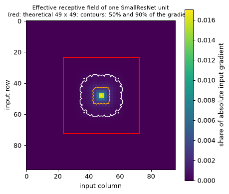
The theoretical window is 49 pixels wide, but about 90% of the gradient lies in the middle 25 pixels, 98% in the middle 33, and the central 9 × 9 pixels alone hold over 40%. The random initialisation gives nearly the same profile. The unit is far more sensitive to the pixels near its centre than to those at the edge of its theoretical field. Gradients through stacked convolutions add up like a sum of random walks, so the weight falls off roughly like a Gaussian, whose width grows only as the square root of the depth. For a task that needs a unit to see an object of a given size, the usable field is smaller than the one the recurrence reports.
Step 6: the gradient at initialisation
The gradient at initialisation shows why depth hurts a plain network. The networks here are small enough to run on 8 × 8 digits: a 3 × 3 stem to 16 channels, then n blocks of two 16-channel 3 × 3 convolutions, then global average pooling and a linear layer. With n = 1, 4, 9, 27 blocks the network has 1 + 2n = 3, 9, 19 and 55 convolution layers. Each is built four ways: with and without identity shortcuts, and with and without batch norm. One forward and backward pass on 256 training images with PyTorch’s default initialisation gives the norm of the gradient that reaches the stem’s weights.
from sklearn.datasets import load_digits
from sklearn.model_selection import train_test_split

digits = load_digits()
X_all = (digits.data / 16.0).astype(np.float32).reshape(-1, 8, 8)
X_tr_raw, X_te_raw, y_tr, y_te = train_test_split(
    X_all, digits.target, test_size=0.25, stratify=digits.target, random_state=0)
mean, std = X_tr_raw.mean(), X_tr_raw.std()
X_tr = torch.from_numpy((X_tr_raw - mean) / std)[:, None]
X_te = torch.from_numpy((X_te_raw - mean) / std)[:, None]
y_tr, y_te = torch.from_numpy(y_tr), torch.from_numpy(y_te)


class DepthBlock(nn.Module):
    """Two 16-channel 3x3 convolutions, with or without BN and an identity shortcut."""
    def __init__(self, width, residual, bn):
        super().__init__()
        self.residual = residual
        self.c1 = nn.Conv2d(width, width, 3, padding=1, bias=not bn)
        self.c2 = nn.Conv2d(width, width, 3, padding=1, bias=not bn)
        self.b1 = nn.BatchNorm2d(width) if bn else nn.Identity()
        self.b2 = nn.BatchNorm2d(width) if bn else nn.Identity()

    def forward(self, x):
        y = self.b2(self.c2(F.relu(self.b1(self.c1(x)))))
        return F.relu(y + x) if self.residual else F.relu(y)


class DepthNet(nn.Module):
    def __init__(self, blocks, residual, bn, width=16):
        super().__init__()
        self.stem = nn.Conv2d(1, width, 3, padding=1, bias=not bn)
        self.stem_bn = nn.BatchNorm2d(width) if bn else nn.Identity()
        self.blocks = nn.Sequential(*[DepthBlock(width, residual, bn) for _ in range(blocks)])
        self.head = nn.Linear(width, 10)

    def forward(self, x):
        x = self.blocks(F.relu(self.stem_bn(self.stem(x))))
        return self.head(x.mean(dim=(2, 3)))


def stem_gradient_norm(blocks, residual, bn):
    torch.manual_seed(0)
    model = DepthNet(blocks, residual, bn).train()
    loss = F.cross_entropy(model(X_tr[:256]), y_tr[:256])
    loss.backward()
    return model.stem.weight.grad.norm().item()


layers = [1 + 2 * n for n in (1, 4, 9, 27)]
print("conv layers:           ", "  ".join(f"{L:9d}" for L in layers))
for bn in (False, True):
    for residual in (False, True):
        norms = [stem_gradient_norm(n, residual, bn) for n in (1, 4, 9, 27)]
        label = f"{'BN' if bn else 'no BN':5s} {'residual' if residual else 'plain':8s}"
        print(f"{label}  stem grad:", "  ".join(f"{v:9.2e}" for v in norms))
conv layers:                    3          9         19         55
no BN plain     stem grad:  5.24e-03   1.41e-05   9.38e-10   0.00e+00
no BN residual  stem grad:  2.18e-02   3.30e-02   5.18e-02   8.71e-02
BN    plain     stem grad:  5.70e-02   9.52e-02   4.99e-01   1.92e+02
BN    residual  stem grad:  7.30e-02   1.76e-01   2.30e-01   7.89e-01
The pattern is the one Section 8 derives. Without normalisation the plain network’s gradient shrinks by a roughly constant factor per layer, which is a geometric decay: PyTorch’s default convolution initialisation draws weights with variance 1/(3\,\text{fan-in}), a sixth of the 2/\text{fan-in} of He initialisation (Module 02, Section 6), so each ReLU layer scales the signal by about 1/\sqrt{6} \approx 0.41, and by 55 layers it has underflowed to zero in float32. Batch norm restores the scale of the forward signal at every layer, and its effect on the backward pass is not benign: in a deep plain network the gradient now explodes instead. Identity shortcuts keep it of order one in both cases, because every block adds an identity term to its Jacobian.
Step 7: the degradation experiment
Now train. Plain and residual networks, both with batch norm, of 7, 19 and 55 convolution layers (n = 3, 9, 27 blocks) are trained on the digits with SGD (momentum 0.9, weight decay 10^{-4}) and a one-cycle cosine schedule that rises to a peak learning rate of 0.05 and falls to nearly zero, batch size 64, 12 epochs, seed 0. The training loss is recorded per epoch, as the mean over the epoch’s mini-batches. At the end each network is evaluated in evaluation mode on the whole training set, to get a training loss that does not depend on the batch statistics of training, and on the test set. If the deeper plain network is worse on the training set, the failure is one of optimisation, not of generalisation: the network is not overfitting, it cannot fit.
def train_depth(blocks, residual, epochs=12, batch=64, peak=0.05, seed=0):
    torch.manual_seed(seed)
    model = DepthNet(blocks, residual, bn=True)
    opt = torch.optim.SGD(model.parameters(), lr=peak, momentum=0.9, weight_decay=1e-4)
    steps = epochs * ((len(X_tr) + batch - 1) // batch)
    sched = torch.optim.lr_scheduler.OneCycleLR(
        opt, max_lr=peak, total_steps=steps, anneal_strategy="cos", cycle_momentum=False)
    g = torch.Generator().manual_seed(seed)
    curve = []
    for _ in range(epochs):
        model.train()
        order = torch.randperm(len(X_tr), generator=g)
        total = 0.0
        for i in range(0, len(X_tr), batch):
            idx = order[i:i + batch]
            opt.zero_grad()
            loss = F.cross_entropy(model(X_tr[idx]), y_tr[idx])
            loss.backward()
            opt.step()
            sched.step()
            total += loss.item() * len(idx)
        curve.append(total / len(X_tr))
    model.eval()
    with torch.no_grad():
        train_loss = F.cross_entropy(model(X_tr), y_tr).item()
        test_acc = (model(X_te).argmax(1) == y_te).float().mean().item()
    return curve, train_loss, test_acc


results = {}
for blocks in (3, 9, 27):
    for residual in (False, True):
        results[(blocks, residual)] = train_depth(blocks, residual)

print("training loss per epoch (mean over mini-batches)")
for (blocks, residual), (curve, _, _) in results.items():
    label = f"{1 + 2 * blocks:2d} layers {'residual' if residual else 'plain   '}"
    print(f"{label}:", " ".join(f"{v:5.2f}" for v in curve))
print()
print("after training, evaluation mode: train loss / test accuracy")
for (blocks, residual), (_, tl, acc) in results.items():
    label = f"{1 + 2 * blocks:2d} layers {'residual' if residual else 'plain   '}"
    print(f"{label}:  {tl:.3f} / {acc:.3f}")
training loss per epoch (mean over mini-batches)
 7 layers plain   :  2.27  1.93  1.31  0.65  0.29  0.46  0.20  0.20  0.12  0.08  0.05  0.05
 7 layers residual:  2.25  1.62  0.75  0.27  0.29  0.25  0.10  0.17  0.10  0.04  0.05  0.04
19 layers plain   :  2.27  1.97  1.69  1.42  1.31  1.13  1.09  0.80  0.60  0.54  0.47  0.43
19 layers residual:  2.41  1.08  0.70  0.38  0.23  0.68  0.25  0.23  0.22  0.08  0.06  0.05
55 layers plain   :  2.27  2.21  2.17  2.13  2.15  2.11  2.11  2.10  2.09  2.09  2.08  2.09
55 layers residual:  2.47  0.83  1.91  1.61  3.00  2.43  0.90  0.75  0.41  0.32  0.32  0.31

after training, evaluation mode: train loss / test accuracy
 7 layers plain   :  0.037 / 0.987
 7 layers residual:  0.034 / 0.984
19 layers plain   :  0.399 / 0.842
19 layers residual:  0.044 / 0.987
55 layers plain   :  2.079 / 0.202
55 layers residual:  0.279 / 0.900
Then the curves, with the loss on a logarithmic axis so that the three scales that matter (about 0.05, 0.5 and 2) are all visible. The dashed line is chance, \ln 10 = 2.30, the loss of a network that always predicts the uniform distribution.
fig, ax = plt.subplots(figsize=(6.4, 4.2))
styles = {3: "tab:blue", 9: "tab:orange", 27: "tab:red"}
for (blocks, residual), (curve, _, _) in results.items():
    ax.plot(range(1, len(curve) + 1), curve, color=styles[blocks],
            linestyle="-" if residual else "--", marker="o" if residual else "s",
            markersize=3, label=f"{1 + 2 * blocks} layers, {'residual' if residual else 'plain'}")
ax.axhline(np.log(10), color="grey", linestyle=":", label="chance (ln 10)")
ax.set_yscale("log")
ax.set_xlabel("epoch")
ax.set_ylabel("training loss (log scale)")
ax.set_title("Degradation: deeper plain networks train worse; residual networks do not")
ax.legend(fontsize=7, ncol=2)
plt.tight_layout()
plt.show()
The deeper plain networks have the higher training loss. At 7 layers the plain and residual networks are alike, both near 0.04. At 19 layers the plain network is already well behind (about 0.4, against 0.04 for the residual one), and at 55 layers it stays near chance, 2.08 against ln 10 = 2.30, after 12 epochs. Its test accuracy, about 20%, is that of a network that has barely learnt anything. Deeper plain networks could, in principle, represent anything the shallower ones can (set the extra layers to the identity); they do not, because optimisation does not find that solution. A residual block makes the identity the default and learning a correction to it the task.
The 55-layer residual network is the one blemish. Its loss jumps up to 3.0 in the middle of the run, when the learning rate is near its peak, and it ends at 0.28 with 90% test accuracy, worse than its shallower siblings: it trains, where the plain network does not, but at this peak learning rate it is not stable. Step 8 asks how much of that is the learning rate.
Step 8: the stability of the deep residual network
Residual connections remove the vanishing gradient, but a 55-layer network has the most layers that can each amplify an update, and a learning rate that suits 7 layers can be too large for it. Train the 55-layer residual network at three peak learning rates and three seeds each, and print the final training loss and test accuracy.
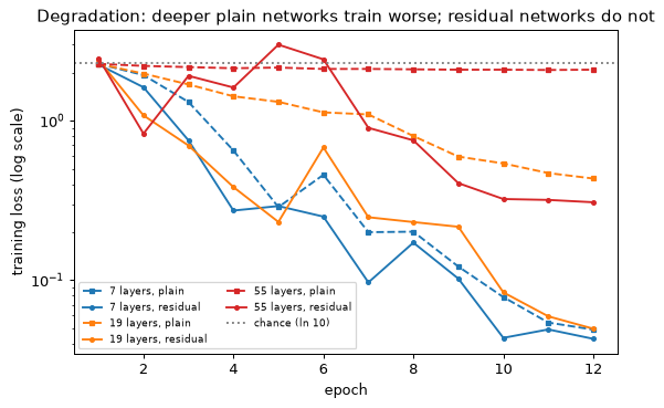
print("55-layer residual network: final train loss / test accuracy, three seeds")
for peak in (0.05, 0.03, 0.02):
    runs = [train_depth(27, True, peak=peak, seed=seed) for seed in range(3)]
    cells = "   ".join(f"{tl:.3f} / {acc:.3f}" for _, tl, acc in runs)
    print(f"peak {peak:.2f}:   {cells}")

print("plain networks at the lower peaks, seed 0: final train loss / test accuracy")
for peak in (0.03, 0.02):
    cells = "   ".join(
        f"{layers} layers {tl:.2f} / {acc:.2f}"
        for layers, (_, tl, acc) in ((2 * b + 1, train_depth(b, False, peak=peak, seed=0))
                                     for b in (9, 27)))
    print(f"peak {peak:.2f}:   {cells}")
55-layer residual network: final train loss / test accuracy, three seeds
peak 0.05:   0.279 / 0.900   0.322 / 0.904   0.105 / 0.938
peak 0.03:   0.061 / 0.969   0.084 / 0.971   0.063 / 0.962
peak 0.02:   0.044 / 0.976   0.052 / 0.967   0.047 / 0.964
plain networks at the lower peaks, seed 0: final train loss / test accuracy
peak 0.03:   19 layers 0.93 / 0.64   55 layers 1.66 / 0.32
peak 0.02:   19 layers 0.88 / 0.68   55 layers 1.91 / 0.27
At the peak of 0.05 the three seeds end at training losses of 0.1 to 0.3; at 0.03 and 0.02 all three are between 0.04 and 0.09 and the test accuracy is 96% to 98%, the level of the shallower residual networks. Lowering the rate does not rescue the plain networks: in the second loop, at peaks of 0.03 and 0.02 their 19-layer training loss is still about 0.9 and their 55-layer loss 1.7 to 1.9, with test accuracy of 0.27 to 0.68. The degradation is a property of the architecture, not of one learning rate. Shortcuts make depth trainable; a modest peak rate, warm-up or zero-initialised branch scales (Try this, 2) make a very deep network stable.
What you should see
- Every hook count matches the formulas of Section 4 and the worked example of Section 8: 1,228,970 parameters and 63,801,856 MACs. A count printed by code is the authority when a hand count and a remembered number disagree.
- The recurrence’s 49 is exactly the extent of the nonzero gradient. Most of the gradient sits in the middle, so the effective receptive field is much smaller than the theoretical one.
- Without normalisation the plain network’s gradient vanishes geometrically with depth. With batch norm alone the deep plain network’s gradient explodes instead. Identity shortcuts keep it of order one in both cases.
- The deeper plain network has a higher training loss, an optimisation failure rather than overfitting, and at 55 layers barely leaves chance (ln 10 = 2.30). The residual versions reach about 0.04 at 7 and 19 layers; at 55 layers they need a lower peak learning rate (0.03 or 0.02) to come down to 0.04–0.08, while no learning rate tried rescues the plain networks.
Try this
- Depthwise-separable blocks. Replace
c1andc2inBlockby a depthwise 3 × 3 followed by a 1 × 1 (call itSepBlock). The parameter count falls from 1,228,970 to 187,018, a factor of 6.6 (the worked example in Section 6; subtract 576 from each count if the stem takes 1 input channel). Train both on the 16 × 16 translated digits of Lab 2 for 10 epochs and compare accuracy and time per epoch. Explain why the time does not fall 6.6-fold: the depthwise layer does little arithmetic per byte moved (Section 6). - Zero-initialised residual branches. Zero the last batch-norm scale of every residual branch
(
nn.init.zeros_(block.b2.weight)) and repeat the 55-layer residual run. Compare the first two epochs with the default: every block starts as the identity. - Plain without batch norm. Remove batch norm and use He initialisation
(
nn.init.kaiming_normal_) in the plain network. How deep can it go before training stalls? - CIFAR-10 at full size. The block below is not run by the lab: it needs
torchvision’s CIFAR-10 loader (a download of about 170 MB) and is best run on a free Google Colab GPU. TrainSmallResNetfor 30 epochs with random crops, horizontal flips and a cosine schedule, with and without augmentation, and plot both validation curves. Nothing else in the module depends on its result.
import torchvision, torchvision.transforms as T
from torch.utils.data import DataLoader

norm = T.Normalize((0.4914, 0.4822, 0.4465), (0.2470, 0.2435, 0.2616))
aug = T.Compose([T.RandomCrop(32, padding=4), T.RandomHorizontalFlip(), T.ToTensor(), norm])
plain = T.Compose([T.ToTensor(), norm])
device = "cuda" if torch.cuda.is_available() else "cpu"


def run(train_tf, epochs=30):
    train = torchvision.datasets.CIFAR10("data", train=True, download=True, transform=train_tf)
    val = torchvision.datasets.CIFAR10("data", train=False, download=True, transform=plain)
    tl = DataLoader(train, batch_size=128, shuffle=True, num_workers=2)
    vl = DataLoader(val, batch_size=512)
    model = SmallResNet().to(device)
    opt = torch.optim.SGD(model.parameters(), lr=0.1, momentum=0.9, weight_decay=5e-4,
                          nesterov=True)
    sched = torch.optim.lr_scheduler.CosineAnnealingLR(opt, epochs * len(tl))
    curve = []
    for _ in range(epochs):
        model.train()
        for xb, yb in tl:
            opt.zero_grad()
            F.cross_entropy(model(xb.to(device)), yb.to(device)).backward()
            opt.step()
            sched.step()
        model.eval()
        with torch.no_grad():
            hits = sum((model(xb.to(device)).argmax(1).cpu() == yb).sum().item()
                       for xb, yb in vl)
        curve.append(hits / len(val))
    return curve


curves = {"augmented": run(aug), "not augmented": run(plain)}
Lab 4 — Transfer learning, layer by layer
Goal. You pretrain a small CNN on the digits 0 to 4 and then adapt it to the digits 5 to 9 from only 5 or 20 labelled images per class. Six ways of doing the adaptation are compared under identical conditions: training from scratch, copying and freezing one, two or three of the three convolutional blocks, and fine-tuning after a frozen start. The comparison shows which layers transfer and which do not, why a frozen backbone can be a poor feature extractor, and how much the gap closes as the target set grows. The last step reproduces the input-normalisation mistake of Section 10, where a perfectly good backbone appears not to transfer at all. The lab needs Section 10 only. The data ships with scikit-learn, there is no download, and the whole lab runs in one to two minutes on a laptop CPU.
Step 1: data, the split and the source and target tasks
The digits are the 8 × 8 images of Lab 2, with the same split: test_size=0.25, stratified,
random_state=0. The source task is the five-way problem on the 675 training images whose
label is 0 to 4. The target task is the five-way problem on digits 5 to 9, and its test set
is the 224 held-out images of those digits. Target training sets are small: 5 or 20 images per
class, drawn from the 672 target training images with a seed, so that five seeds give five
different small sets from the same pool.
All images are standardised with the mean and standard deviation of the source training set. That is the rule of Section 10: the backbone is trained on inputs with these statistics, so it must see inputs with these statistics, whatever task follows. Step 7 shows what happens when this is forgotten.
import time
import numpy as np
import torch
import torch.nn as nn
import torch.nn.functional as F
import matplotlib.pyplot as plt
from sklearn.datasets import load_digits
from sklearn.model_selection import train_test_split

np.random.seed(0)
torch.manual_seed(0)
torch.set_num_threads(4)

X, y = load_digits(return_X_y=True)
X = (X / 16.0).astype(np.float32).reshape(-1, 1, 8, 8)
Xtr, Xte, ytr, yte = train_test_split(X, y, test_size=0.25, stratify=y, random_state=0)

src_tr, src_te = ytr < 5, yte < 5
mean, std = Xtr[src_tr].mean(), Xtr[src_tr].std()  # source statistics, used everywhere
Z_tr = torch.from_numpy((Xtr - mean) / std)
Z_te = torch.from_numpy((Xte - mean) / std)
y_tr, y_te = torch.from_numpy(ytr), torch.from_numpy(yte)

print(f"source: {src_tr.sum()} train, {src_te.sum()} test (digits 0-4)")
print(f"target: {(~src_tr).sum()} train pool, {(~src_te).sum()} test (digits 5-9)")
print(f"source mean {mean:.4f}, std {std:.4f}")
source: 675 train, 226 test (digits 0-4)
target: 672 train pool, 224 test (digits 5-9)
source mean 0.3052, std 0.3782
Step 2: the backbone
The backbone has three blocks, each a convolution, batch normalisation and ReLU. The first block sees pixels and can only compute local patterns: strokes and edges. The second adds a max pool, which halves the map to 4 × 4, and mixes those into short curves and corners. The third widens to 64 channels and ends in global average pooling, so the backbone’s output is a vector of 64 numbers per image. A linear layer on top is the head. Keeping the three blocks as separate modules makes it possible to copy, freeze or re-initialise any prefix of the backbone.
The parameter count is exact arithmetic. Block 1: 1 \cdot 16 \cdot 9 + 16 = 160 convolution parameters and 2 \cdot 16 = 32 for batch norm. Block 2: 16 \cdot 32 \cdot 9 + 32 = 4{,}640 and 64. Block 3: 32 \cdot 64 \cdot 9 + 64 = 18{,}496 and 128. The sum is 23,520, and the code prints the same figure; the head adds 64 \cdot 5 + 5 = 325.
def block(c_in, c_out, pool=False, gap=False):
    layers = [nn.Conv2d(c_in, c_out, 3, padding=1), nn.BatchNorm2d(c_out), nn.ReLU()]
    if pool:
        layers.append(nn.MaxPool2d(2))
    if gap:
        layers += [nn.AdaptiveAvgPool2d(1), nn.Flatten()]
    return nn.Sequential(*layers)


class Net(nn.Module):
    """Three feature blocks and a linear head; each block can be copied or frozen."""

    def __init__(self, n_classes):
        super().__init__()
        self.blocks = nn.ModuleList([block(1, 16), block(16, 32, pool=True),
                                     block(32, 64, gap=True)])
        self.head = nn.Linear(64, n_classes)

    def features(self, x):
        for b in self.blocks:
            x = b(x)
        return x

    def forward(self, x):
        return self.head(self.features(x))


n_backbone = sum(p.numel() for p in Net(5).blocks.parameters())
print(f"backbone parameters: {n_backbone:,}; head: {64 * 5 + 5}")
backbone parameters: 23,520; head: 325
Step 3: one training function for every variant
All six experiments are the same loop with different parts frozen, so the loop is written once.
fit takes a model, a training set, a number of epochs, a learning rate and the number of
frozen blocks at the front. Three details are the ones that go wrong in practice:
- Frozen parameters get
requires_grad = False, and the optimiser is given only the parameters that are still trainable, so no update can touch the frozen blocks. - Freezing parameters does not freeze batch-normalisation statistics. In training mode a
batch-norm layer updates its running mean and variance on every forward pass, so a “frozen”
block would quietly drift towards the target data. The frozen blocks must be put back into
eval()mode after every call tomodel.train(). - The target labels 5 to 9 are mapped to 0 to 4 for the new five-way head.
def set_frozen(model, n_frozen):
    for i, b in enumerate(model.blocks):
        for p in b.parameters():
            p.requires_grad = i >= n_frozen


def fit(model, X, y, epochs, lr, n_frozen=0, batch=32, seed=0):
    """Train with Adam; the first n_frozen blocks are frozen, in eval mode."""
    set_frozen(model, n_frozen)
    params = [p for p in model.parameters() if p.requires_grad]
    opt = torch.optim.Adam(params, lr=lr)
    g = torch.Generator().manual_seed(seed)
    n = len(X)
    for _ in range(epochs):
        model.train()
        for i in range(n_frozen):
            model.blocks[i].eval()          # keeps the batch-norm statistics fixed
        perm = torch.randperm(n, generator=g)
        for k in range(0, n, batch):
            idx = perm[k:k + batch]
            loss = F.cross_entropy(model(X[idx]), y[idx])
            opt.zero_grad()
            loss.backward()
            opt.step()
    model.eval()
    return model


@torch.no_grad()
def accuracy(model, X, y):
    model.eval()
    return (model(X).argmax(1) == y).float().mean().item()
Step 4: pretrain on the source task
Thirty epochs of Adam at 3 \times 10^{-3} on 675 images take a few seconds. The source test set is the 226 held-out images of digits 0 to 4. Five digit classes of this kind are easy, so the accuracy should be close to 1; the pretraining only has to work, not to be interesting.
t0 = time.time()
source = Net(5)
fit(source, Z_tr[src_tr], y_tr[src_tr], epochs=30, lr=3e-3)
print(f"source test accuracy: {accuracy(source, Z_te[src_te], y_te[src_te]):.3f}")
source test accuracy: 1.000
Step 5: six ways to adapt to digits 5 to 9
Each variant builds a new network with a fresh five-way head and copies some blocks from the pretrained one:
| Name | Blocks copied | Frozen during stage 1 | Stage 2 |
|---|---|---|---|
| (a) scratch | none | none | none |
| (b) block 1 | 1 | 1 | none |
| (c) blocks 1-2 | 1, 2 | 1, 2 | none |
| (d) probe | 1, 2, 3 | 1, 2, 3 | none |
| (e) probe + fine-tune | 1, 2, 3 | 1, 2, 3 | all blocks, 3 \times 10^{-4} |
| (f) block 1 + fine-tune | 1 | 1 | all blocks, 3 \times 10^{-4} |
Variant (d) is the linear probe: with every block frozen, the only thing learned is a linear classifier on the 64 pooled features. Variants (e) and (f) follow the schedule of Section 10: train the new parts at a normal rate, then unfreeze everything and train at a tenth of that rate, so that the copied weights move gently. Stage 1 uses 100 epochs at 3 \times 10^{-3} with a batch of 16, and the fine-tuning stage another 100 epochs.
target_set draws n images per class with a given seed from the target training pool and
subtracts 5 from the labels. run_variant returns the target test accuracy.
tgt_idx = np.where(~src_tr)[0]


def target_set(n_per_class, seed):
    rng = np.random.default_rng(seed)
    pick = []
    for c in range(5, 10):
        pool = tgt_idx[ytr[tgt_idx] == c]
        pick += list(rng.choice(pool, n_per_class, replace=False))
    pick = np.array(pick)
    return Z_tr[pick], y_tr[pick] - 5


te_mask = torch.from_numpy(~src_te)
Zt_te, yt_te = Z_te[te_mask], y_te[te_mask] - 5


def run_variant(name, Xs, ys, seed):
    """Adapt `source` to the target task in one of six ways; return test accuracy."""
    torch.manual_seed(seed)
    model = Net(5)                                  # fresh head, fresh random blocks
    n_copy = {"a": 0, "b": 1, "c": 2, "d": 3, "e": 3, "f": 1}[name]
    for i in range(n_copy):
        model.blocks[i].load_state_dict(source.blocks[i].state_dict())
    kw = dict(epochs=100, lr=3e-3, batch=16, seed=seed)
    fit(model, Xs, ys, n_frozen=n_copy, **kw)
    if name in ("e", "f"):
        fit(model, Xs, ys, n_frozen=0, **{**kw, "lr": 3e-4})
    return accuracy(model, Zt_te, yt_te)


Xs, ys = target_set(5, seed=0)
print("target training set:", tuple(Xs.shape), "labels:", torch.bincount(ys).tolist())
t0 = time.time()
print(f"scratch, seed 0, n = 5: {run_variant('a', Xs, ys, 0):.3f}")
target training set: (25, 1, 8, 8) labels: [5, 5, 5, 5, 5]
scratch, seed 0, n = 5: 0.897
Step 6: the experiment, five seeds, two sizes
The comparison runs every variant at n = 5 and n = 20 for seeds 0 to 4. With 25 or 100 training images the target test accuracy depends noticeably on which images were drawn, so a single seed would be a coin toss. Five seeds give a mean and a spread; with a spread of two to three points, differences of one point between variants are noise and are not interpreted. The table lists the mean and the standard deviation (over seeds) of the accuracy on the 224 target test images.
names = {"a": "scratch", "b": "block 1 frozen", "c": "blocks 1-2 frozen",
         "d": "linear probe (1-3)", "e": "probe, then fine-tune",
         "f": "block 1, then fine-tune"}
results = {}
t0 = time.time()
for n in (5, 20):
    for v in names:
        accs = []
        for seed in range(5):
            Xs, ys = target_set(n, seed)
            accs.append(run_variant(v, Xs, ys, seed))
        results[(n, v)] = np.array(accs)

print(f"{'variant':27s} {'n = 5':>14s} {'n = 20':>14s}")
for v, label in names.items():
    cells = [f"{results[(n, v)].mean():.3f} +/- {results[(n, v)].std():.3f}"
             for n in (5, 20)]
    print(f"({v}) {label:23s} {cells[0]:>14s} {cells[1]:>14s}")
variant                              n = 5         n = 20
(a) scratch                 0.913 +/- 0.021 0.969 +/- 0.007
(b) block 1 frozen          0.909 +/- 0.033 0.966 +/- 0.019
(c) blocks 1-2 frozen       0.873 +/- 0.032 0.959 +/- 0.034
(d) linear probe (1-3)      0.662 +/- 0.033 0.762 +/- 0.010
(e) probe, then fine-tune   0.807 +/- 0.022 0.960 +/- 0.007
(f) block 1, then fine-tune 0.902 +/- 0.029 0.981 +/- 0.011
The same numbers as a plot make the ordering and the size of the error bars easier to judge.
fig, axes = plt.subplots(1, 2, figsize=(10, 3.8), sharey=True)
for ax, n in zip(axes, (5, 20)):
    means = [results[(n, v)].mean() for v in names]
    sds = [results[(n, v)].std() for v in names]
    ax.bar(range(6), means, yerr=sds, capsize=3, color="#4c78a8")
    ax.set_xticks(range(6))
    ax.set_xticklabels([f"({v})" for v in names])
    ax.set_title(f"{n} labelled images per class")
    ax.set_xlabel("variant")
    ax.set_ylim(0.4, 1.0)
axes[0].set_ylabel("target test accuracy (mean, sd over 5 seeds)")
fig.suptitle("Digits 5-9 after pretraining on digits 0-4")
plt.tight_layout()
plt.show()
Step 7: the normalisation mistake
Variant (d) is the most sensitive to input statistics, since nothing downstream can adapt to them. The experiment trains the linear probe at n = 10 per class and evaluates it twice: on target test images standardised with the source statistics, as in training, and on raw [0, 1] pixels. This is what happens when a deployed model is fed inputs preprocessed differently from its training pipeline: a pretrained backbone assumes an input scale, and everything after it is calibrated to that scale.
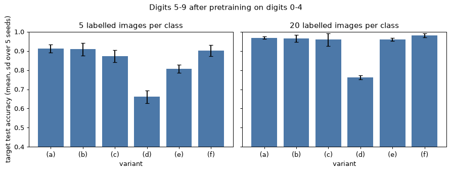
raw_te = torch.from_numpy(Xte)[te_mask]
ok, bad = [], []
for seed in range(5):
    Xs, ys = target_set(10, seed)
    torch.manual_seed(seed)
    model = Net(5)
    for i in range(3):
        model.blocks[i].load_state_dict(source.blocks[i].state_dict())
    fit(model, Xs, ys, epochs=100, lr=3e-3, batch=16, n_frozen=3, seed=seed)
    ok.append(accuracy(model, Zt_te, yt_te))
    bad.append(accuracy(model, raw_te, yt_te))
print(f"probe, standardised inputs (correct): {np.mean(ok):.3f} +/- {np.std(ok):.3f}")
print(f"probe, raw [0,1] pixels  (mistake)  : {np.mean(bad):.3f} +/- {np.std(bad):.3f}")
probe, standardised inputs (correct): 0.713 +/- 0.013
probe, raw [0,1] pixels  (mistake)  : 0.209 +/- 0.016
What you should see
- The source task is learned, the target is not free. The pretrained network reaches 1.000 on the 226 source test images, yet its frozen features are a poor basis for digits 5 to 9. The linear probe (d) reaches about 0.66 at n = 5 and 0.76 at n = 20, while a network trained from scratch on the same images reaches about 0.91 and 0.97. The last block was trained to separate 0, 1, 2, 3 and 4. Its 64 pooled features keep what those five classes need and discard what 5 to 9 need, and more labels cannot bring the discarded information back. Early layers are general and later layers are specific (Section 10; Yosinski et al., 2014). A narrow source transfers little more than its first block, and ImageNet’s breadth is the reason a whole ImageNet backbone transfers.
- The first block transfers harmlessly, not usefully. Copying and freezing block 1 (b) matches scratch within the seed spread at both sizes (0.909 against 0.913, 0.966 against 0.969). Its 3 × 3 stroke and edge detectors are as good as ones learned from 25 images, but with only 16 \cdot 9 = 144 weights they are also cheap to learn, so little is gained. Freezing blocks 1 and 2 (c) is slightly worse at n = 5 (0.873): block 2’s features are already specific to the source digits. The ordering by depth of what is copied, (b) then (c) then (d), is the observation; the one-point differences between (a) and (b) are not.
- Fine-tuning recovers most of the loss, and the gap closes with data. The probe followed by fine-tuning (e) rises from 0.662 to 0.807 at n = 5 and from 0.762 to 0.960 at n = 20, where it is within about a point of scratch. At n = 5 it still trails scratch by about 10 points: 25 images are too few to move a backbone that starts in a bad place. Block 1 followed by fine-tuning (f) is as good as scratch at n = 5 (0.902) and the best variant at n = 20 (0.981 against 0.969), but the difference to scratch at n = 20 is about one standard deviation of the seed spread, so it is a hint and not a result. At n = 20 everything except the probe is within a few points of everything else.
- The normalisation mistake looks like a failure to transfer. On correctly standardised inputs the probe scores about 0.71 at n = 10. Fed raw [0, 1] pixels, whose mean is 0.31 and standard deviation 0.38 instead of 0 and 1, it falls to about 0.21, chance for five classes. Nothing is wrong with the backbone, the weights or the code; the inputs are on a scale that the batch-norm layers and the frozen head were not calibrated for. This is the “transfer learning does not work” report of Section 10, and the check is two lines: print the mean and standard deviation of what the model is fed and compare them with those of its training pipeline.
- Noise sets the scale of every claim. The standard deviations over seeds range from 0.007 to 0.034. Rerun with other seeds and the last digits will change; the ordering of the probe below everything else, and of the collapse on raw pixels, will not.
Try this
- Discriminative learning rates. Fine-tune with 3 \times 10^{-5}, 10^{-4} and 3 \times 10^{-4} for blocks 1, 2 and 3 and 3 \times 10^{-3} for the head, using one parameter group per block in Adam, and compare with variant (e).
- The batch-norm trap. Remove the line that puts the frozen blocks back into
eval()mode. Print one batch-norm layer’srunning_meanbefore and after training the head, and compare the accuracy of the probe. The “frozen” backbone is no longer the pretrained one. - Where the source matters. Pretrain on digits 0 to 4 placed at random positions on the 16 × 16 canvas of Lab 2, repeat the six variants on the canvas, and compare the linear probe with scratch training that re-samples positions. The lesson is the same: a probe on features that were specific to the source stays weak.
- A broad source. The block below is not executed here, because it needs
torchvisionand a 44.7 MB download of ImageNet weights. Run it on Colab to see a broad source transfer its whole backbone: a probe on the 512-dimensional pooled features is far stronger than the probe of this lab. No number in this module depends on it.
import torchvision
from torchvision.models import resnet18

net = resnet18(weights="IMAGENET1K_V1").eval()
net.fc = torch.nn.Identity()                          # 512-dimensional pooled features
mean_in = torch.tensor([0.485, 0.456, 0.406]).view(1, 3, 1, 1)
std_in = torch.tensor([0.229, 0.224, 0.225]).view(1, 3, 1, 1)


def imagenet_features(x_8x8):                         # (N, 1, 8, 8) in [0, 1]
    x = F.interpolate(torch.from_numpy(x_8x8), size=64, mode="bilinear")
    x = x.repeat(1, 3, 1, 1)                          # grey to three channels
    with torch.no_grad():
        return net((x - mean_in) / std_in)            # ImageNet's own statistics

# then: logistic regression on imagenet_features(...) for n = 5 per class (variant d),
# a small network from scratch (variant a), and fine-tuning the whole net (variant e).
Lab 5 — U-Net segmentation on synthetic images, and from mask to measurement
Goal. You train a small U-Net to segment the circles, and only the circles, in synthetic
microscopy-like images that also contain rectangles of the same brightness. You first show that
a global intensity threshold cannot do the job, then measure what the U-Net’s skip connections
contribute by training it twice, with and without them, and score both with the Dice coefficient
and the intersection over union (Section 12). Finally you turn the predicted masks into
measurements, area and perimeter, and compare them with the true circles. This is the
two-dimensional version of the mask-to-surface step of Section 13: the area behaves
like a volume, the perimeter like a surface area, and the way the perimeter is measured matters
more than the network. The data is generated in NumPy and there is no download. In full mode the
whole lab takes about two minutes on a desktop CPU and two to four minutes on a
laptop; set QUICK = True in the first block for a run of about 15 seconds in all, at the
price of a worse and noisier result.
Step 1: the synthetic images
Each image is 64 × 64 and contains two to four objects, each a circle (radius 4 to 10 pixels) or a rectangle (sides 6 to 18 pixels), with intensities drawn from the same range, 0.5 to 1.0. Objects may overlap, and a later object overwrites an earlier one. The image is then blurred with a Gaussian of standard deviation 1 pixel, as an optical system would blur it, a linear illumination ramp of amplitude up to 0.3 is added in a random direction, and Gaussian noise of standard deviation 0.1 is added on top. The target mask contains the circles only.
Two conventions matter later for the measurements. Pixel (i, j) has its centre at (i + 0.5,\; j + 0.5), and a pixel belongs to a circle if its centre lies inside the circle. The generator also returns the list of isolated circles: those that are not overwritten by any later object and have no other object within 3 pixels. Only these have a clean ground-truth area \pi r^2 and perimeter 2\pi r for step 8.
import time
import numpy as np
import torch
import torch.nn as nn
import torch.nn.functional as F
import matplotlib.pyplot as plt
from scipy import ndimage as ndi
import contourpy

QUICK = False                     # True: 400 images x 8 epochs, about 7 s per model
N_TRAIN, EPOCHS = (400, 8) if QUICK else (1500, 15)
SIZE = 64

np.random.seed(0)
torch.manual_seed(0)
torch.set_num_threads(4)

YY, XX = np.mgrid[0:SIZE, 0:SIZE] + 0.5          # pixel centres at (i + 0.5, j + 0.5)


def make_image(rng):
    """One image, its circle mask and the list of isolated circles (cy, cx, r)."""
    ids = np.zeros((SIZE, SIZE), dtype=int)       # object id per pixel, 0 = background
    img = np.zeros((SIZE, SIZE))
    kinds, discs = [None], [None]
    for k in range(1, rng.integers(2, 5) + 1):
        value = rng.uniform(0.5, 1.0)
        if rng.random() < 0.5:
            r = rng.uniform(4, 10)
            cy, cx = rng.uniform(r + 2, SIZE - r - 2, 2)
            m = (YY - cy) ** 2 + (XX - cx) ** 2 <= r * r
            kinds.append("circle")
            discs.append((cy, cx, r, m))
        else:
            h, w = rng.uniform(6, 18, 2)
            y0, x0 = rng.uniform(2, SIZE - h - 2), rng.uniform(2, SIZE - w - 2)
            m = (YY >= y0) & (YY < y0 + h) & (XX >= x0) & (XX < x0 + w)
            kinds.append("rect")
            discs.append(None)
        img[m] = value
        ids[m] = k
    mask = np.isin(ids, [k for k in range(1, len(kinds)) if kinds[k] == "circle"])
    circles = []
    for k in range(1, len(kinds)):
        if kinds[k] != "circle":
            continue
        cy, cx, r, m = discs[k]
        other = (ids > 0) & (ids != k)
        whole = (ids == k).sum() == m.sum()          # not overwritten by a later object
        if whole and not (ndi.binary_dilation(m, iterations=3) & other).any():
            circles.append((cy, cx, r))
    img = ndi.gaussian_filter(img, 1.0)
    theta, amp = rng.uniform(0, 2 * np.pi), rng.uniform(0, 0.3)
    u = ((XX - SIZE / 2) * np.cos(theta) + (YY - SIZE / 2) * np.sin(theta))
    img = img + amp * u / (SIZE / 2 * (abs(np.cos(theta)) + abs(np.sin(theta))))
    img = img + rng.normal(0, 0.1, img.shape)
    return img.astype(np.float32), mask, circles


def make_dataset(n, seed):
    rng = np.random.default_rng(seed)
    out = [make_image(rng) for _ in range(n)]
    return (np.stack([o[0] for o in out]), np.stack([o[1] for o in out]),
            [o[2] for o in out])


Xtr, Ytr, _ = make_dataset(N_TRAIN, seed=0)
Xva, Yva, circ_va = make_dataset(200, seed=1)
print("train:", Xtr.shape, Ytr.shape, " val:", Xva.shape)
print(f"foreground fraction: train {Ytr.mean():.3f}, val {Yva.mean():.3f}")
print(f"isolated circles in the validation set: {sum(len(c) for c in circ_va)}")
train: (1500, 64, 64) (1500, 64, 64)  val: (200, 64, 64)
foreground fraction: train 0.056, val 0.056
isolated circles in the validation set: 161
The foreground fraction near 6% means that 94% of pixels are background, so pixel accuracy would be 94% for a model that predicts nothing. That is why segmentation is scored with overlap measures, and why Step 4 adds a Dice term to the loss. A look at eight images first.
fig, axes = plt.subplots(2, 8, figsize=(14, 3.8))
for k in range(8):
    axes[0, k].imshow(Xtr[k], cmap="gray", vmin=0, vmax=1.2)
    axes[1, k].imshow(Ytr[k], cmap="gray")
    axes[0, k].axis("off")
    axes[1, k].axis("off")
axes[0, 0].set_title("image", loc="left")
axes[1, 0].set_title("target mask (circles only)", loc="left")
fig.suptitle("Synthetic training images: circles are targets, rectangles distract")
plt.tight_layout()
plt.show()
Step 2: a threshold baseline
Before any network, the simplest segmenter: call a pixel foreground if its intensity exceeds a global threshold. The threshold is chosen to maximise Dice on 300 training images, scanning 33 values from 0.1 to 0.9, and then evaluated on the validation set. The metrics are pooled over all pixels of all images,
with P the predicted foreground and T the target. A threshold sees one pixel at a time, so it cannot tell a circle from a rectangle of the same brightness, and the illumination ramp shifts brightness across the image. The best it can do is segment objects, both kinds, as well as the ramp allows, and the rectangles then count as false positives.
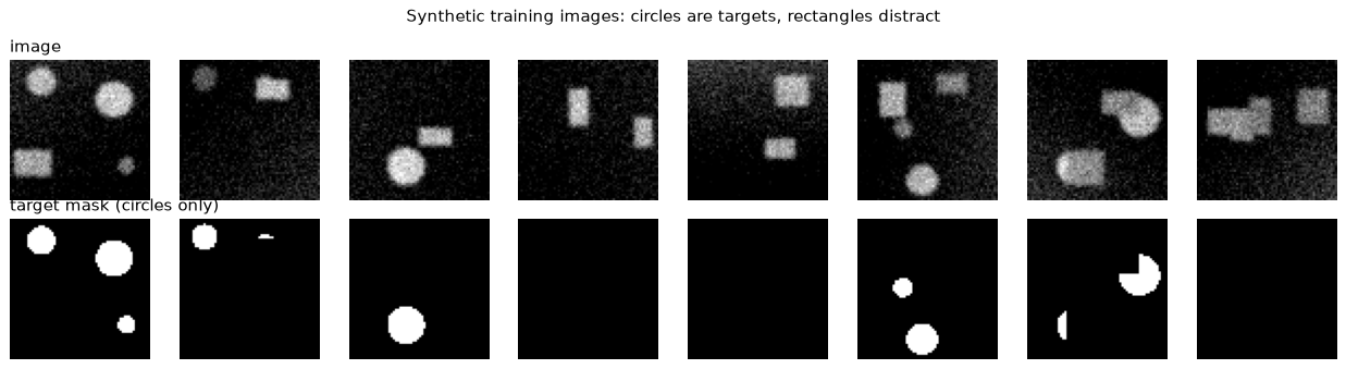
def dice_iou(pred, target):
    """Pooled Dice and IoU over all pixels of boolean arrays."""
    inter = np.logical_and(pred, target).sum()
    union = np.logical_or(pred, target).sum()
    return 2 * inter / (pred.sum() + target.sum()), inter / union


ths = np.linspace(0.1, 0.9, 33)
scores = [dice_iou(Xtr[:300] > t, Ytr[:300])[0] for t in ths]
th = ths[int(np.argmax(scores))]
d, j = dice_iou(Xva > th, Yva)
print(f"best threshold {th:.2f} (train Dice {max(scores):.3f});"
      f" validation Dice {d:.3f}, IoU {j:.3f}")
best threshold 0.40 (train Dice 0.662); validation Dice 0.641, IoU 0.471
Step 3: the U-Net
The network follows Section 12. cbr is the unit of the design: two convolutions, each
followed by batch normalisation and ReLU, with the bias dropped because batch norm’s offset
makes it redundant. The encoder has three levels, at 64 × 64, 32 × 32 and 16 × 16, with channels
8, 16 and 32 and a 2 × 2 max pool between levels. The bottleneck at 8 × 8 has 64 channels. The
decoder mirrors the encoder: a transposed convolution with kernel 2 and stride 2 doubles the
resolution and halves the channels, the result is concatenated with the encoder map of the
same resolution, and a cbr mixes them. A final 1 × 1 convolution gives one logit per pixel.
With skips=False the concatenations are dropped, and the decoder’s convolutions take half as
many input channels. The two models differ only in whether the decoder can see the encoder’s
full-resolution maps.
The pooling steps need the input to be divisible by 2^3 = 8, which 64 is.
def cbr(c_in, c_out):
    return nn.Sequential(
        nn.Conv2d(c_in, c_out, 3, padding=1, bias=False),
        nn.BatchNorm2d(c_out), nn.ReLU(),
        nn.Conv2d(c_out, c_out, 3, padding=1, bias=False),
        nn.BatchNorm2d(c_out), nn.ReLU())


class UNet(nn.Module):
    def __init__(self, c=(8, 16, 32, 64), skips=True):
        super().__init__()
        self.skips = skips
        m = 2 if skips else 1                       # decoder input: upsampled (+ skip)
        self.enc = nn.ModuleList([cbr(1, c[0]), cbr(c[0], c[1]), cbr(c[1], c[2])])
        self.bott = cbr(c[2], c[3])
        self.up = nn.ModuleList([nn.ConvTranspose2d(c[3], c[2], 2, 2),
                                 nn.ConvTranspose2d(c[2], c[1], 2, 2),
                                 nn.ConvTranspose2d(c[1], c[0], 2, 2)])
        self.dec = nn.ModuleList([cbr(m * c[2], c[2]), cbr(m * c[1], c[1]),
                                  cbr(m * c[0], c[0])])
        self.out = nn.Conv2d(c[0], 1, 1)

    def forward(self, x):
        saved = []
        for enc in self.enc:
            x = enc(x)
            saved.append(x)                         # full-resolution maps for the skips
            x = F.max_pool2d(x, 2)
        x = self.bott(x)
        for up, dec in zip(self.up, self.dec):
            x = up(x)
            if self.skips:
                x = torch.cat([x, saved.pop()], dim=1)
            else:
                saved.pop()
            x = dec(x)
        return self.out(x)


for sk in (True, False):
    n_par = sum(p.numel() for p in UNet(skips=sk).parameters())
    print(f"skips={sk!s:5}: {n_par:,} parameters")
print("output shape:", tuple(UNet()(torch.zeros(2, 1, 64, 64)).shape))
skips=True : 121,033 parameters
skips=False: 108,937 parameters
output shape: (2, 1, 64, 64)
The model with skips has 12,096 more parameters, all in the decoder’s first convolutions, which now read twice as many channels. Skip connections are cheap in parameters. Their cost is memory: the encoder maps must be kept until the decoder uses them.
Step 4: loss, training loop and metrics
The loss is the sum of binary cross-entropy on the logits and a soft Dice loss. Cross-entropy gives a well-behaved gradient for every pixel but is dominated by the 94% background. The soft Dice loss, 1 - (2\sum p\,t + \epsilon)/(\sum p + \sum t + \epsilon) with p the predicted probability, t the target and \epsilon = 1, optimises overlap directly and does not care about the class balance. It is computed per image and averaged, so that a small circle counts as much as a large one.
Training uses Adam with a one-cycle learning-rate schedule (10% warm-up to a peak of 3 \times 10^{-3}, then cosine decay) and batches of 16. Every third epoch the loop prints the training loss and three validation numbers at threshold 0.5: Dice and IoU pooled over all pixels, and the boundary-band accuracy, the pixel accuracy inside a band of ±2 pixels around the true boundaries, obtained as binary dilation minus binary erosion of the target mask with a two-dimensional cross as the structuring element. Overall Dice is dominated by object interiors, which are easy. The band is where the models differ.
cross = np.zeros((3, 3, 3), dtype=bool)
cross[1] = ndi.generate_binary_structure(2, 1)      # 2D cross, per image
BAND = (ndi.binary_dilation(Yva, cross, iterations=2)
        & ~ndi.binary_erosion(Yva, cross, iterations=2))
print(f"band covers {BAND.mean():.3f} of the validation pixels")


def loss_fn(logits, target):
    bce = F.binary_cross_entropy_with_logits(logits, target)
    p = torch.sigmoid(logits)
    inter = (p * target).sum((1, 2, 3))
    dice = (2 * inter + 1) / (p.sum((1, 2, 3)) + target.sum((1, 2, 3)) + 1)
    return bce + (1 - dice).mean()


@torch.no_grad()
def predict(model, X, batch=100):
    model.eval()
    xs = torch.from_numpy(X)[:, None]
    return torch.cat([torch.sigmoid(model(xs[i:i + batch]))[:, 0]
                      for i in range(0, len(X), batch)]).numpy()


def evaluate(model):
    prob = predict(model, Xva)
    pred = prob > 0.5
    d, j = dice_iou(pred, Yva)
    return d, j, (pred == Yva)[BAND].mean()


def train(model, epochs=EPOCHS, bs=16, max_lr=3e-3, report=3):
    xs = torch.from_numpy(Xtr)[:, None]
    ys = torch.from_numpy(Ytr.astype(np.float32))[:, None]
    steps = epochs * int(np.ceil(len(xs) / bs))
    opt = torch.optim.Adam(model.parameters(), lr=max_lr)
    sched = torch.optim.lr_scheduler.OneCycleLR(opt, max_lr=max_lr, total_steps=steps,
                                                pct_start=0.1)
    g = torch.Generator().manual_seed(0)
    for ep in range(1, epochs + 1):
        model.train()
        perm = torch.randperm(len(xs), generator=g)
        total = 0.0
        for k in range(0, len(xs), bs):
            idx = perm[k:k + bs]
            loss = loss_fn(model(xs[idx]), ys[idx])
            opt.zero_grad()
            loss.backward()
            opt.step()
            sched.step()
            total += loss.item() * len(idx)
        if ep % report == 0 or ep == epochs:
            d, j, b = evaluate(model)
            print(f"  epoch {ep:2d}  loss {total / len(xs):.3f}  val Dice {d:.3f}"
                  f"  IoU {j:.3f}  band acc {b:.3f}")
    return model
band covers 0.054 of the validation pixels
Step 5: train with and without skip connections
The two runs use the same seed, data, schedule and batch order. Only skips differs. In full
mode each takes about 40 to 60 seconds on a four-thread desktop CPU.
models, final = {}, {}
for skips in (True, False):
    torch.manual_seed(0)
    t0 = time.time()
    print(f"U-Net, skips={skips}")
    models[skips] = train(UNet(skips=skips))
    final[skips] = evaluate(models[skips])

print()
print(f"{'':14s} {'Dice':>6s} {'IoU':>6s} {'band acc':>9s}")
print(f"{'threshold':14s} {d:6.3f} {j:6.3f} {'-':>9s}")
for skips, label in ((True, "U-Net, skips"), (False, "U-Net, no skips")):
    dd, jj, bb = final[skips]
    print(f"{label:14s} {dd:6.3f} {jj:6.3f} {bb:9.3f}")
U-Net, skips=True
  epoch  3  loss 0.447  val Dice 0.930  IoU 0.870  band acc 0.930
  epoch  6  loss 0.161  val Dice 0.836  IoU 0.718  band acc 0.901
  epoch  9  loss 0.083  val Dice 0.957  IoU 0.918  band acc 0.934
  epoch 12  loss 0.063  val Dice 0.965  IoU 0.932  band acc 0.948
  epoch 15  loss 0.057  val Dice 0.965  IoU 0.933  band acc 0.950
U-Net, skips=False
  epoch  3  loss 0.681  val Dice 0.875  IoU 0.778  band acc 0.850
  epoch  6  loss 0.265  val Dice 0.912  IoU 0.838  band acc 0.850
  epoch  9  loss 0.105  val Dice 0.939  IoU 0.885  band acc 0.900
  epoch 12  loss 0.073  val Dice 0.949  IoU 0.903  band acc 0.913
  epoch 15  loss 0.064  val Dice 0.952  IoU 0.908  band acc 0.920

                 Dice    IoU  band acc
threshold       0.641  0.471         -
U-Net, skips    0.965  0.933     0.950
U-Net, no skips  0.952  0.908     0.920
The decoder without skips has to rebuild boundaries from an 8 × 8 bottleneck, where each unit covers an 8 × 8 pixel block. It can place an object and get its shape roughly right, but fine position information at the resolution of single pixels has been pooled away. Skip connections hand it that information back.
The next figure shows four validation images, the target, and both predictions at threshold 0.5. The differences between the two models sit along the boundaries.
prob = {k: predict(m, Xva[:4]) for k, m in models.items()}
fig, axes = plt.subplots(4, 4, figsize=(9, 9))
cols = ["image", "target", "with skips", "without skips"]
for r in range(4):
    axes[r, 0].imshow(Xva[r], cmap="gray", vmin=0, vmax=1.2)
    axes[r, 1].imshow(Yva[r], cmap="gray")
    axes[r, 2].imshow(prob[True][r] > 0.5, cmap="gray")
    axes[r, 3].imshow(prob[False][r] > 0.5, cmap="gray")
    for c in range(4):
        axes[r, c].axis("off")
        if r == 0:
            axes[r, c].set_title(cols[c])
fig.suptitle("Validation images: input, target and the two U-Nets' predictions")
plt.tight_layout()
plt.show()
Step 6: Dice and IoU are the same ranking
For a single image with a = |P \cap T|, |P| + |T| = a + u where u = |P \cup T| (since |P| + |T| = |P \cup T| + |P \cap T|), so \text{Dice} = 2a/(a + u) and \text{IoU} = a/u. Substituting a = \text{IoU} \cdot u gives
The relation is monotone, so the two metrics rank any set of models identically; they differ only in scale, and Dice is the larger. The check below verifies the identity numerically, image by image and for the pooled pair. Report one of them, say which, and do not compare a Dice from one paper with an IoU from another.
pred = predict(models[True], Xva) > 0.5
per_image = []
for p_i, t_i in zip(pred, Yva):
    if p_i.sum() + t_i.sum() == 0:
        continue                                    # both empty: 0/0
    d_i, j_i = dice_iou(p_i, t_i)
    per_image.append(abs(d_i - 2 * j_i / (1 + j_i)))
d_all, j_all = dice_iou(pred, Yva)
print(f"images checked: {len(per_image)}, "
      f"max |Dice - 2 IoU/(1+IoU)| = {max(per_image):.1e}")
print(f"pooled: Dice {d_all:.4f}, IoU {j_all:.4f}, "
      f"2 IoU/(1+IoU) = {2 * j_all / (1 + j_all):.4f}")
images checked: 166, max |Dice - 2 IoU/(1+IoU)| = 1.1e-16
pooled: Dice 0.9651, IoU 0.9325, 2 IoU/(1+IoU) = 0.9651
Step 7: connected components and the isolated circles
To measure objects, the binary prediction is split into connected components with
ndi.label, which assigns an integer to each group of touching foreground pixels. For each of
the isolated true circles in the validation set, the matching prediction is the component that
contains the circle’s centre pixel. A circle whose centre is background in the prediction is
counted as missed. Two measurements follow, each divided by the exact value for the true
circle, so that 1.0 means unbiased:
- Area is the number of pixels of the component, against \pi r^2.
- Perimeter is measured in two ways. (a) The number of pixel edges between foreground and
background, the crudest way of measuring the boundary of a mask. (b) The length of the
iso-contour at level 0.5 of the predicted probability, which
contourpycomputes with marching squares, the two-dimensional relative of marching cubes: it interpolates along each cell edge to find where the probability crosses 0.5, and joins the crossings into polylines. The probability map is zeroed outside a two-pixel margin around the component, so that the contour belongs to this component only. Both are compared with 2\pi r.
prob_va = predict(models[True], Xva)
bin_va = prob_va > 0.5
rows = []
for i in range(len(Xva)):
    labels, _ = ndi.label(bin_va[i])
    for cy, cx, r in circ_va[i]:
        lab = labels[int(cy), int(cx)]                 # component at the centre pixel
        if lab == 0:
            rows.append((np.nan, np.nan, np.nan))
            continue
        comp = labels == lab
        padded = np.pad(comp, 1).astype(int)
        edges = (np.abs(np.diff(padded, axis=0)).sum()
                 + np.abs(np.diff(padded, axis=1)).sum())
        z = prob_va[i] * ndi.binary_dilation(comp, iterations=2)
        lines = contourpy.contour_generator(z=z).lines(0.5)
        length = sum(np.hypot(*np.diff(np.asarray(ln), axis=0).T).sum() for ln in lines)
        rows.append((comp.sum() / (np.pi * r * r), edges / (2 * np.pi * r),
                     length / (2 * np.pi * r)))
rows = np.array(rows)
found = ~np.isnan(rows[:, 0])
print(f"isolated circles: {len(rows)}, found by the U-Net: {found.sum()}")
for name, col in (("area / (pi r^2)", 0), ("pixel-edge perimeter / (2 pi r)", 1),
                  ("iso-contour perimeter / (2 pi r)", 2)):
    v = rows[found, col]
    print(f"{name:34s} mean {v.mean():.3f}  sd {v.std():.3f}")

fig, axes = plt.subplots(1, 3, figsize=(11, 3.4))
titles = ("area", "pixel-edge perimeter", "iso-contour perimeter")
for ax, col, name in zip(axes, range(3), titles):
    ax.hist(rows[found, col], bins=25, color="#4c78a8")
    ax.axvline(1.0, color="k", lw=1)
    ax.set_title(name)
    ax.set_xlabel("measured / true")
axes[0].set_ylabel("circles")
fig.suptitle("Measurements from predicted masks, relative to the true circles")
plt.tight_layout()
plt.show()
isolated circles: 161, found by the U-Net: 160
area / (pi r^2)                    mean 0.999  sd 0.029
pixel-edge perimeter / (2 pi r)    mean 1.266  sd 0.035
iso-contour perimeter / (2 pi r)   mean 1.033  sd 0.017
The standard deviation of the area ratio, a few per cent, is the variance of the measurement: how much one circle’s predicted area differs from another’s. The mean of the perimeter ratios is the bias: for the pixel-edge perimeter it is about 27% and nothing the network does can change it. This is the error decomposition of Module 01 in a form that can be measured, and the reason for step 8.
Step 8: why the pixel-edge perimeter is 27% too long
Take the best mask any network could return: an ideal digital disc, the set of pixels whose centres lie within a circle of radius r. Its pixel-edge perimeter is the length of a staircase. A staircase approximating a curve covers the same horizontal and vertical extent as the curve, so its length is the sum of the extents, not the arclength: over a quarter circle that is 2r, over the whole circle 8r, against 2\pi r. The ratio is 4/\pi = 1.273 at every radius, however fine the grid. Counting edges is therefore biased by 27% at any resolution; this is a property of the measure, not of the image.
The test below uses discs of radius 4, 8, 16 and 24 at a sub-pixel offset, and three measures of the boundary: pixel edges, marching squares on the binary mask (level 0.5), and marching squares on a mask blurred with a Gaussian of standard deviation 1, which is what a smooth probability map from a network looks like.
def disc(r, size=128, offset=(0.3, 0.4)):
    c = size / 2 + np.array(offset)
    yy, xx = np.mgrid[0:size, 0:size] + 0.5
    return ((yy - c[0]) ** 2 + (xx - c[1]) ** 2 <= r * r).astype(float)


def edge_count(mask):
    p = np.pad(mask, 1)
    return np.abs(np.diff(p, axis=0)).sum() + np.abs(np.diff(p, axis=1)).sum()


def contour_length(z):
    lines = contourpy.contour_generator(z=z).lines(0.5)
    return sum(np.hypot(*np.diff(np.asarray(ln), axis=0).T).sum() for ln in lines)


print(f"{'r':>3s} {'pixel edges':>12s} {'squares, binary':>16s}"
      f" {'squares, blurred':>17s}")
for r in (4, 8, 16, 24):
    m = disc(r)
    print(f"{r:3d} {edge_count(m) / (2 * np.pi * r):12.3f}"
          f" {contour_length(m) / (2 * np.pi * r):16.3f}"
          f" {contour_length(ndi.gaussian_filter(m, 1.0)) / (2 * np.pi * r):17.3f}")
  r  pixel edges  squares, binary  squares, blurred
  4        1.273            1.040             0.972
  8        1.273            1.052             0.996
 16        1.273            1.052             1.003
 24        1.273            1.056             1.005
Marching squares on the binary mask does better than the edge count, because its vertices sit at the midpoints of the cell edges and cut the corners of the staircase, but a binary input gives it nothing finer than half a pixel to interpolate with. On a smooth probability map the interpolation recovers the sub-pixel position of the boundary, and the error falls to within about one per cent for radii of 8 and above. The smallest disc is 3% short, because blurring moves the 0.5 level of a small disc inwards. This is the mechanism that Section 13 uses in three dimensions: counting exposed voxel faces is biased high by a constant factor, and marching cubes on a smooth field is not.
What you should see
- A threshold cannot do this task. The best global threshold (0.40) reaches Dice 0.641 and IoU 0.471 on the validation images, and its training Dice (0.662) is no better, so this is a limit of the method and not overfitting. A pixel’s intensity says nothing about whether the object it belongs to is round. The U-Net reaches Dice 0.965 because its bottleneck units each see an area of the image larger than an object, so they can compute shape.
- Skip connections matter at the boundary more than overall. With skips: Dice 0.965, IoU 0.933, boundary-band accuracy 0.950. Without: 0.952, 0.908, 0.920. Overall Dice moves by 1.3 points and band accuracy by 3.0, and the band gap is visible at every reported epoch while the pooled Dice is not (epoch 6 of the skip model even dips to 0.836, while the learning rate is still high, and recovers). Dice is dominated by object interiors, where both models are right. The decoder alone cannot recover detail lost in the 8 × 8 bottleneck. This is one run per model: the band ordering holds at every reported epoch, but a difference of one Dice point would need several seeds before it was believed. Expect larger gaps in QUICK mode, where the decoder without skips has less time to compensate.
- Dice and IoU are one ranking. The identity \text{Dice} = 2\,\text{IoU}/(1 + \text{IoU}) holds to round-off (10^{-16}) on every image and for the pooled pair (0.9651 both ways). The models are ordered the same way by either.
- Pixel counts are unbiased; pixel-edge perimeters are not. Over 160 of the 161 isolated circles (one was missed), the area ratio has mean 0.999 and standard deviation 0.029. The pixel-edge perimeter ratio has mean 1.266, close to 4/\pi = 1.273, with standard deviation 0.035: the bias is almost the whole error. The iso-contour of the predicted probability gives 1.033 with standard deviation 0.017, a bias of 3% and half the spread. Step 8 shows that on ideal discs the pixel-edge ratio is exactly 1.273 at every radius, marching squares on a binary mask is 4 to 6% high, and on a blurred mask it is within 1% for r \geq 8.
- What this means for volumes and surfaces. The same pattern holds in 3D (Section 13): voxel counts give volumes with small bias, face counts overstate surface areas by a constant factor that depends on orientation, and an isosurface of a smooth field is the accurate measure. A good Dice score says little about the second of these.
Try this
- Checkerboards. Replace
ConvTranspose2d(k=2, s=2)byConvTranspose2d(k=3, s=2, padding=1, output_padding=1)and look for a checkerboard pattern in the predicted probabilities early in training. With kernel 3 and stride 2 the output pixels receive different numbers of contributions, which is the cause (Section 12). Then usenn.Upsample(scale_factor=2, mode="bilinear")followed by a 3 × 3 convolution and compare. - Losses. Train with BCE only and with Dice only. Compare Dice on the small circles (radius below 6) and the training curves; one of the two is typically slower to start.
- Input size. Feed a 100 × 100 image to the trained U-Net. Explain the error (three poolings need a multiple of 8, and the skips need matching shapes) and fix it by padding to 104 and cropping the output.
- Three dimensions. Rebuild the network with
Conv3dand theDown3Dblock of Section 13, usingGroupNorm(8, C)in place of batch norm, on synthetic 32³ volumes of spheres and cubes. Measure the volumes by voxel count, as in step 7, and compare the time per epoch with the 2D model.
Lab 6 — Grad-CAM catches a shortcut
Goal. You train two small CNNs to tell circles from squares. One is trained on data in which every square carries a small bright marker in the top-left corner, so the marker predicts the class perfectly; the other is trained on clean data. Both score well on data drawn like their training set, and only a test set in which the marker no longer predicts the class exposes the difference. You then implement a saliency map and Grad-CAM from their definitions (Section 14), see where each model looks, verify that Grad-CAM for a global-average-pooling head is the class activation map of Zhou et al., and run the model-randomisation sanity check of Adebayo et al. The data is synthetic, there is no download, and the lab runs in about ten seconds on a laptop CPU.
Step 1: images with and without a shortcut
Each image is 32 × 32 and holds one shape, a circle with radius or a square with half-side drawn
from 5 to 9 pixels, at a random position that keeps it clear of the top-left corner, with
intensity 0.6 to 1.0, a Gaussian blur of standard deviation 0.7 pixels and noise of standard
deviation 0.1. The marker is a 3 × 3 patch of intensity 1.0 at rows and columns 1 to 3. The
rule argument of make decides where it appears:
"spurious": on every square and on no circle, so the marker is a perfect predictor;"none": never, the clean data;"random": on a random half of the images, independent of the class.
Training sets of 2,000 images are made with the first two rules (seed 0). Test sets of 500 are made with seed 1 (clean) and seed 2 (random marker), and a further 500 images with the spurious rule (seed 3) play the part of the validation set that a developer would normally look at: drawn from the training distribution.
import copy
import numpy as np
import torch
import torch.nn as nn
import torch.nn.functional as F
import matplotlib.pyplot as plt
from scipy import ndimage as ndi

np.random.seed(0)
torch.manual_seed(0)
torch.set_num_threads(4)

S = 32
YY, XX = np.mgrid[0:S, 0:S] + 0.5


def shape_img(rng, cls, marker):
    """cls 0 = circle, 1 = square; marker adds the 3x3 corner patch."""
    img = np.zeros((S, S))
    a = rng.uniform(5, 9)
    cy, cx = rng.uniform(a + 4, S - a - 2, 2)           # clear of the top-left corner
    if cls == 0:
        m = (YY - cy) ** 2 + (XX - cx) ** 2 <= a * a
    else:
        m = (np.abs(YY - cy) <= a) & (np.abs(XX - cx) <= a)
    img[m] = rng.uniform(0.6, 1.0)
    if marker:
        img[1:4, 1:4] = 1.0
    img = ndi.gaussian_filter(img, 0.7) + rng.normal(0, 0.1, img.shape)
    return img.astype(np.float32)


def make(n, seed, rule):
    rng = np.random.default_rng(seed)
    y = rng.integers(0, 2, n)
    if rule == "spurious":
        marker = y == 1
    elif rule == "none":
        marker = np.zeros(n, dtype=bool)
    else:
        marker = rng.random(n) < 0.5
    X = np.stack([shape_img(rng, c, m) for c, m in zip(y, marker)])
    return torch.from_numpy(X)[:, None], torch.from_numpy(y), marker


Xs_tr, ys_tr, _ = make(2000, 0, "spurious")
Xc_tr, yc_tr, _ = make(2000, 0, "none")
Xs_va, ys_va, _ = make(500, 3, "spurious")
Xc_te, yc_te, _ = make(500, 1, "none")
Xr_te, yr_te, mr_te = make(500, 2, "random")
print("train:", tuple(Xs_tr.shape), f" class balance: {ys_tr.float().mean().item():.3f}")
print(f"random-marker test set: marker on {mr_te.mean():.2f} of images,"
      f" on {mr_te[yr_te.numpy() == 1].mean():.2f} of squares and"
      f" {mr_te[yr_te.numpy() == 0].mean():.2f} of circles")

fig, axes = plt.subplots(2, 8, figsize=(13, 3.6))
for r, (X, y, name) in enumerate([(Xs_tr, ys_tr, "spurious"), (Xc_tr, yc_tr, "clean")]):
    for k in range(8):
        axes[r, k].imshow(X[k, 0], cmap="gray", vmin=0, vmax=1.2)
        axes[r, k].set_title(["circle", "square"][int(y[k])], fontsize=9)
        axes[r, k].axis("off")
    axes[r, 0].text(-0.15, 0.5, name, transform=axes[r, 0].transAxes, rotation=90,
                    va="center", ha="right")
fig.suptitle("Training images: marker on every square (top), clean (bottom)")
plt.tight_layout()
plt.show()
train: (2000, 1, 32, 32)  class balance: 0.521
random-marker test set: marker on 0.49 of images, on 0.52 of squares and 0.47 of circles
Step 2: the network
The network is deliberately small and ends the way a classic CNN does: global average pooling
over the last convolutional map and one linear layer. forward returns the logits and the last
convolutional map A, of shape (B, 32, 16, 16), because Grad-CAM needs to differentiate with
respect to it. Parameter count: 160 + 4{,}640 + 9{,}248 + 66 = 14{,}114.
class Net(nn.Module):
    def __init__(self):
        super().__init__()
        self.c1 = nn.Conv2d(1, 16, 3, padding=1)
        self.c2 = nn.Conv2d(16, 32, 3, padding=1)
        self.c3 = nn.Conv2d(32, 32, 3, padding=1)
        self.fc = nn.Linear(32, 2)

    def forward(self, x):
        x = F.max_pool2d(F.relu(self.c1(x)), 2)         # 16 x 16
        x = F.relu(self.c2(x))
        A = F.relu(self.c3(x))                          # last conv map (B, 32, 16, 16)
        return self.fc(A.mean((2, 3))), A


def train(X, y, epochs=8, bs=64, lr=2e-3, seed=0):
    torch.manual_seed(seed)
    model = Net()
    opt = torch.optim.Adam(model.parameters(), lr=lr)
    g = torch.Generator().manual_seed(seed)
    for _ in range(epochs):
        model.train()
        perm = torch.randperm(len(X), generator=g)
        for k in range(0, len(X), bs):
            idx = perm[k:k + bs]
            loss = F.cross_entropy(model(X[idx])[0], y[idx])
            opt.zero_grad()
            loss.backward()
            opt.step()
    return model.eval()


@torch.no_grad()
def acc(model, X, y):
    return (model(X)[0].argmax(1) == y).float().mean().item()


print("parameters:", sum(p.numel() for p in Net().parameters()))
parameters: 14114
Step 3: validation accuracy that hides the shortcut
Train both models and score each on three test sets: the validation set drawn like the shortcut training data, the clean test set, and the random-marker test set. The question is what each number would tell a developer who only ever looked at the first one.
shortcut = train(Xs_tr, ys_tr)
clean = train(Xc_tr, yc_tr)

print(f"{'':18s} {'marker = class':>15s} {'clean':>7s} {'random marker':>14s}")
for name, m in (("shortcut model", shortcut), ("clean model", clean)):
    print(f"{name:18s} {acc(m, Xs_va, ys_va):15.3f} {acc(m, Xc_te, yc_te):7.3f}"
          f" {acc(m, Xr_te, yr_te):14.3f}")
                    marker = class   clean  random marker
shortcut model               1.000   0.750          0.718
clean model                  0.986   0.984          0.958
The shortcut model scores 1.000 on data drawn like its training set, 0.750 on clean data and 0.718 when the marker is decorrelated from the class. Its first score is perfect because the marker alone gives the answer; the second shows that it learned the shapes only partly, because the marker left little pressure to learn them. On the clean set the marker is missing for every square, and with balanced classes 0.750 is what labelling every circle right and half the squares gives. The clean model scores 0.984 on clean data. Its 0.986 on the first set says that a marker on squares does not confuse it, and its 0.958 on the random-marker set says that a marker on circles confuses it a little: the marker is a bright patch it never saw. Nothing in the first column of the table reveals the difference between the two models. Only a test set in which the shortcut breaks, or a look inside, does.
Step 4: saliency and Grad-CAM from the definitions
Both methods answer “where is the evidence for class c?”, and both start from the logit y^c of the class, before the softmax.
The saliency map is the magnitude of the gradient of the logit with respect to the input pixels, |\partial y^c / \partial x_{ij}|: the pixels where a small change would move the score most. It has the resolution of the image and is noisy, because the gradient of a ReLU network is a piecewise-constant function of the input.
Grad-CAM works on the last convolutional map instead. For each channel k it computes the weight \alpha_k^c, the gradient of y^c with respect to that channel’s map averaged over its Z = H \cdot W positions, and forms the weighted sum, keeping only the positive evidence:
The result has the resolution of A (16 × 16 here) and is upsampled bilinearly to the image
size for display. In code, A.retain_grad() makes PyTorch keep the gradient of this
intermediate tensor, and backward on the single logit fills it.
The quantity to read from either map is the share of its total mass inside the top-left 6 × 6 corner, which holds the marker and a margin around it, and is 36/1024 = 3.5\% of the image. A map that ignores the corner would put about 3.5% of its mass there. The test images are 100 squares from the random-marker set that carry the marker, the class is square, and the same images go to both models.
def grad_cam(model, x, c):
    """Grad-CAM for class c on one image x of shape (1, 1, S, S); returns (S, S)."""
    logits, A = model(x)
    A.retain_grad()
    logits[0, c].backward()
    alpha = A.grad.mean((2, 3), keepdim=True)       # (1, K, 1, 1): mean over positions
    cam = F.relu((alpha * A).sum(1, keepdim=True)).detach()
    up = F.interpolate(cam, size=(S, S), mode="bilinear", align_corners=False)
    return up[0, 0].numpy()


def saliency(model, x, c):
    x = x.clone().requires_grad_(True)
    model(x)[0][0, c].backward()
    return x.grad.abs()[0, 0].numpy()


def corner_share(m):
    return m[:6, :6].sum() / (m.sum() + 1e-12)


idx = np.where(mr_te & (yr_te.numpy() == 1))[0][:100]
share = {}
for name, model in (("shortcut", shortcut), ("clean", clean)):
    xs = [Xr_te[i:i + 1] for i in idx]
    share[name] = (np.mean([corner_share(grad_cam(model, x, 1)) for x in xs]),
                   np.mean([corner_share(saliency(model, x, 1)) for x in xs]))
print(f"{len(idx)} squares carrying the marker; "
      f"the corner is {36 / S ** 2:.3f} of the image")
print(f"{'':16s} {'Grad-CAM share':>15s} {'saliency share':>15s}")
for name, (g, s) in share.items():
    print(f"{name + ' model':16s} {g:15.3f} {s:15.3f}")
100 squares carrying the marker; the corner is 0.035 of the image
                  Grad-CAM share  saliency share
shortcut model             0.269           0.088
clean model                0.101           0.061
Step 5: look at the maps
The grid shows one square with the marker, the two models in the two rows, and for each the input with its Grad-CAM overlaid and the saliency map. Titles state the corner share of that image’s map.
i0 = int(idx[0])
x0 = Xr_te[i0:i0 + 1]
fig, axes = plt.subplots(2, 3, figsize=(9, 6))
pair = (("shortcut model", shortcut), ("clean model", clean))
for r, (name, model) in enumerate(pair):
    cam, sal = grad_cam(model, x0, 1), saliency(model, x0, 1)
    axes[r, 0].imshow(x0[0, 0], cmap="gray", vmin=0, vmax=1.2)
    axes[r, 0].set_title(f"{name}: input")
    axes[r, 1].imshow(x0[0, 0], cmap="gray", vmin=0, vmax=1.2)
    axes[r, 1].imshow(cam, cmap="jet", alpha=0.5)
    axes[r, 1].set_title(f"Grad-CAM, corner share {corner_share(cam):.2f}")
    axes[r, 2].imshow(sal, cmap="hot")
    axes[r, 2].set_title(f"saliency, corner share {corner_share(sal):.2f}")
    for c in range(3):
        axes[r, c].axis("off")
fig.suptitle("Evidence for 'square': shortcut model (top), clean model (bottom)")
plt.tight_layout()
plt.show()
Step 6: Grad-CAM with a pooling head is the CAM
For this architecture the weights \alpha_k^c do not need backpropagation. The logit is y^c = \sum_k w_k^c \cdot \frac{1}{Z}\sum_{i,j} A^k_{ij} + b^c, which is linear in A, so
Since the factor 1/Z scales the whole map and the display normalises it, Grad-CAM equals the
class activation map of Zhou et al. (2016), \sum_k w_k^c A^k, the head’s weights applied
at every position. Grad-CAM’s contribution was to extend the idea to networks with any head, by
replacing w_k^c/Z with the gradient. The check uses the trained shortcut model and reads the
number of positions from the map itself, A.shape[2] * A.shape[3].
x = Xr_te[i0:i0 + 1]
logits, A = shortcut(x)
A.retain_grad()
logits[0, 1].backward()
alpha = A.grad.mean((2, 3))[0]
Z = A.shape[2] * A.shape[3]
w = shortcut.fc.weight[1].detach()
print(f"Z = {Z}; max |alpha - w_c / Z| = {(alpha - w / Z).abs().max().item():.1e}")
Z = 256; max |alpha - w_c / Z| = 2.3e-10
Step 7: a randomisation test of the map
A heatmap can look plausible and still not explain anything: edge detectors, for instance, give
object-shaped maps whether or not a network is involved. Adebayo et al. (2018) proposed a
necessary condition. Destroy the learned weights of the layers closest to the output, and the
map must change. The test copies the shortcut model, re-initialises its head and its last
convolution with reset_parameters(), recomputes Grad-CAM on the same 100 images and prints the
mean Pearson correlation between each pair of maps. A correlation near 1 would mean that the
method ignores the weights.
broken = copy.deepcopy(shortcut)
broken.fc.reset_parameters()
broken.c3.reset_parameters()

corrs = []
for i in idx:
    a = grad_cam(shortcut, Xr_te[i:i + 1], 1).ravel()
    b = grad_cam(broken, Xr_te[i:i + 1], 1).ravel()
    if a.std() > 0 and b.std() > 0:
        corrs.append(np.corrcoef(a, b)[0, 1])
print(f"maps compared: {len(corrs)}; mean correlation trained vs re-initialised: "
      f"{np.mean(corrs):.2f}")
shares = [corner_share(grad_cam(broken, Xr_te[i:i + 1], 1)) for i in idx]
print(f"corner share after re-initialisation: {np.mean(shares):.3f}")
maps compared: 100; mean correlation trained vs re-initialised: 0.18
corner share after re-initialisation: 0.015
What you should see
- Validation accuracy drawn from the training distribution says nothing about the shortcut. The shortcut model scores 1.000 there and 0.750 on clean data, a gap of 25 points, while the clean model scores 0.986 and 0.984. A developer who looked only at the first column would ship the shortcut model. The remedy is a test set built to break the suspected shortcut, here the random-marker set (0.718 against 0.958), and not more of the same validation data.
- Grad-CAM points at the marker for the shortcut model. Averaged over 100 marker-carrying squares, 0.269 of the shortcut model’s Grad-CAM mass falls in the 6 × 6 corner that is 3.5% of the image, about 8 times its share of the area, against 0.101 for the clean model. The saliency shares are 0.088 and 0.061, in the same direction and much less decisive, which is the usual verdict on raw gradients: they are noisy, and the difference between the models is within what one would hesitate to call a finding. In the example of Step 5 both models also respond to the square’s top and bottom edges, so the shortcut model uses the marker and some shape evidence, which fits its 0.750 on clean data; the figure does not show a model that looks only at the marker.
- The clean model’s corner share is not 3.5% either. At 0.101 it is about three times the area share, because a marker is a bright, sharp-cornered patch and the clean model’s edge-and-corner detectors respond to it. A heat map is evidence about the model’s response to this input, and a small non-zero share in a place that should not matter is a reason to test with the marker removed, not a conclusion.
- With a global-average-pooling head, Grad-CAM is CAM. The weights \alpha_k^c agree with w_k^c/Z for Z = 256 to 2 \times 10^{-10}, float32 round-off, so the gradient computation reproduces the closed form of Step 6.
- The map depends on the model. After re-initialising the head and the last convolution, the mean correlation with the trained model’s map is 0.18, and the corner share falls to 0.015. This is necessary evidence that the method responds to the learned weights; it is not sufficient evidence that the map explains the model, since a method could pass this test and still mislead. Occlusion (Try this 1) is an independent check that uses no gradients.
Try this
- Occlusion. Slide a 6 × 6 grey patch (the image mean) over a marker-carrying square, record the drop in the class score at each position, and plot it as a map. It needs no gradients at all; compare it with Grad-CAM, and with saliency, on both models.
- Resolution. Compute Grad-CAM on the digit CNN of Lab 2. Its last convolutional map is 4 × 4 and the images are 8 × 8, so the heat map has at most 16 cells, and explain why the result is too coarse to say where in a digit the evidence lies.
- Remove the correlation. Retrain the shortcut model on a training set in which the marker
appears on a random half of all images (rule
"random") and confirm that its Grad-CAM mass in the corner falls, and that its clean accuracy rises. Then ask what else in the data could still be a shortcut, such as the area difference between a circle and a square of the same radius, and design a test that would show it.
Exercises
Fifteen exercises, graded by the effort they ask for. A one-star exercise (★) is conceptual and takes about five minutes: answer it in a few sentences. A two-star exercise (★★) is a derivation or a calculation of about ten minutes, to be done on paper with a calculator. The one three-star exercise (★★★) is a project of about 25 minutes that needs code. There are seven of the first kind (35 minutes), seven of the second (70 minutes) and one of the third, 130 minutes in all. The study plan places each exercise after the reading it tests, so that no reading block runs on without something to do.
Attempt every exercise before you open its solution. The solutions are hidden until you open them, and they are written to be read in full: each gives the answer first, then every step and the reason for taking it, and every number in them was computed and checked. Where a solution includes code, the code was run and the output shown is what it printed; the last digits may differ on your machine. If your answer differs from the solution’s, find the first line where the two part company before you read on. A wrong number with a correct method is usually a slip. A correct number reached by a different method is worth comparing with the solution’s, because the difference often shows an assumption. The exercises use numbers of their own: none repeats a worked example or a check from the text, apart from Exercises 4 and 8, which refer to results of Lab 2 and Lab 4.
Output sizes, and the rows a window never reads. A 7 × 7 single-channel input is convolved with a 3 × 3 kernel. Padding p, stride s and dilation d are the same along both axes.
(a) Give the output size for (p, s, d) = (0,1,1), (1,1,1), (1,2,1), (0,1,2) and (0,2,2).
(b) For the two stride-2 cases, list the input rows that each output row reads. Which input rows, if any, are never read?
(c) What padding keeps the output at 7 × 7 with dilation 2 and stride 1?
Show solution
(a) The sizes. The formula of Section 3 counts window positions. A window of a 3 \times 3 kernel with dilation d spans d(k-1) + 1 cells; after padding the axis has H + 2p cells. Windows start at cells 0, s, 2s, \dots, and the last start is the one that still leaves room for the span, at H + 2p - d(k-1) - 1. Counting the starts gives
With H = 7 and k = 3 the numerator is 7 + 2p - 2d - 1 = 6 + 2p - 2d:
| (p, s, d) | span | numerator | output size |
|---|---|---|---|
| (0, 1, 1) | 3 | 4 | \lfloor 4/1 \rfloor + 1 = 5 |
| (1, 1, 1) | 3 | 6 | \lfloor 6/1 \rfloor + 1 = 7 |
| (1, 2, 1) | 3 | 6 | \lfloor 6/2 \rfloor + 1 = 4 |
| (0, 1, 2) | 5 | 2 | \lfloor 2/1 \rfloor + 1 = 3 |
| (0, 2, 2) | 5 | 2 | \lfloor 2/2 \rfloor + 1 = 2 |
The sizes are 5, 7, 4, 3 and 2, along each axis, so the outputs are 5 \times 5, 7 \times 7, 4 \times 4, 3 \times 3 and 2 \times 2.
(b) What the stride-2 windows read. Work in padded coordinates, where padded cell q is input row q - p; cells that fall outside 0, \dots, 6 are padding.
- (1, 2, 1): the padded axis has 9 cells, 0 to 8. Windows start at 0, 2, 4, 6 and read the padded cells \{0,1,2\}, \{2,3,4\}, \{4,5,6\} and \{6,7,8\}. Subtracting p = 1, the output rows read the input rows \{-1,0,1\}, \{1,2,3\}, \{3,4,5\} and \{5,6,7\}, where -1 and 7 are padding. Every input row is read. Rows 1, 3 and 5 are read twice, because a window of width 3 at stride 2 overlaps its neighbour by k - s = 1 row; rows 0, 2, 4 and 6 are read once.
- (0, 2, 2): no padding, and each window spans 5 cells. Windows start at 0 and 2 (the next start, 4, would end at row 8). Their taps are rows \{0, 2, 4\} and \{2, 4, 6\}. Rows 1, 3 and 5 are never read.
The second case is not an accident of the size. Every window starts at a multiple of the stride, t = s m, and reads t, t + d, t + 2d, so every row it reads is a multiple of \gcd(s, d). Here \gcd(2, 2) = 2 and only even rows are visible. It is the same defect as the gridding of a dilated stack in Section 3, arriving through the stride instead of through repeated dilations. In two dimensions it is worse: only the 16 pixels with both coordinates even are read, a third of the 49.
(c) ‘Same’ padding with dilation. Stride 1 and a numerator of H - 1 keep the size, so H + 2p - d(k-1) - 1 = H - 1, which gives p = d(k-1)/2. With d = 2 and k = 3 that is p = 2, and indeed \lfloor (7 + 4 - 4 - 1)/1 \rfloor + 1 = 7. The span of the dilated kernel is 5, so it needs the same border as a 5 \times 5 kernel.
The loop below checks all of it with PyTorch. It runs one axis as a 1D convolution of ones and reads off the gradient of the output’s sum with respect to each input cell, which is the number of windows that read it.
import torch
import torch.nn as nn

def rows_read(h, k, p, s, d):
    """Output length, and how many windows read each input row (one axis)."""
    conv = nn.Conv1d(1, 1, k, stride=s, padding=p, dilation=d, bias=False)
    nn.init.ones_(conv.weight)
    x = torch.ones(1, 1, h, requires_grad=True)
    y = conv(x)
    y.sum().backward()          # d(sum y)/dx[i] = number of windows that read x[i]
    return y.shape[-1], x.grad[0, 0].int().tolist()

for p, s, d in [(0, 1, 1), (1, 1, 1), (1, 2, 1), (0, 1, 2), (0, 2, 2), (2, 1, 2)]:
    size, counts = rows_read(7, 3, p, s, d)
    print(f"p={p} s={s} d={d}: output {size}, reads per row {counts}")
p=0 s=1 d=1: output 5, reads per row [1, 2, 3, 3, 3, 2, 1]
p=1 s=1 d=1: output 7, reads per row [2, 3, 3, 3, 3, 3, 2]
p=1 s=2 d=1: output 4, reads per row [1, 2, 1, 2, 1, 2, 1]
p=0 s=1 d=2: output 3, reads per row [1, 1, 2, 1, 2, 1, 1]
p=0 s=2 d=2: output 2, reads per row [1, 0, 2, 0, 2, 0, 1]
p=2 s=1 d=2: output 7, reads per row [2, 2, 3, 3, 3, 2, 2]
The output sizes agree with the formula, the rows read by (1, 2, 1) and (0, 2, 2) are the ones listed above, and the last line is part (c). A shape that comes out right does not show that every input was used: the (0, 2, 2) layer returns a perfectly ordinary 2 \times 2 map while ignoring two thirds of its input.
Three ways to a 9 × 9 receptive field. (a) Show that n stacked k \times k convolutions with stride 1 have the receptive field of a single convolution of size n(k-1) + 1.
(b) With C input and C output channels in every layer and no biases, compare three ways of reaching a 9 \times 9 field: one 9 \times 9 layer, two 5 \times 5 layers and four 3 \times 3 layers. Count the weights, the multiply-accumulates per output position and the nonlinearities (one after each layer).
(c) Generalise to n stacked 3 \times 3 layers against one (2n+1) \times (2n+1) layer. What fraction of the weights does the stack use as n grows, and what does it give up?
Show solution
(a) The field of a stack. Work along one axis. A single layer’s unit reads k consecutive inputs, so r_1 = k. Suppose a unit of layer n - 1 depends on a window of r_{n-1} consecutive inputs. A unit of layer n reads k adjacent units of layer n - 1, and adjacent units have windows shifted by one input, because the stride is 1. The union of k windows of width r_{n-1}, each shifted by one cell from the last, is a window of width r_{n-1} + (k - 1). So r_n = r_{n-1} + (k - 1), which is the recurrence of Section 3 with every jump equal to 1 and every dilation equal to 1. Starting from r_0 = 1 (a unit sees only itself),
For k = 3 this is 2n + 1, for k = 5 it is 4n + 1, and a 9 \times 9 field needs n(k-1) = 8: (k, n) = (9, 1), (5, 2) or (3, 4).
(b) The three designs. A k \times k layer with C channels in and out has k^2 C^2 weights. At stride 1 with ‘same’ padding it computes one output vector at every position, and each weight is used once per position, so the multiply-accumulates per output position equal the weights (Section 4):
| Design | Field | Weights | MACs per position | Nonlinearities |
|---|---|---|---|---|
| one 9 \times 9 | 9 | 81\,C^2 | 81\,C^2 | 1 |
| two 5 \times 5 | 9 | 2 \cdot 25\,C^2 = 50\,C^2 | 50\,C^2 | 2 |
| four 3 \times 3 | 9 | 4 \cdot 9\,C^2 = 36\,C^2 | 36\,C^2 | 4 |
For concreteness take C = 32 on a 40 \times 40 map (1,600 positions): the weights are 82,944, 51,200 and 36,864, and the layers cost 132.7, 81.9 and 59.0 million MACs. The deepest stack is the cheapest, with less than half the weights of the single layer, and it has the most nonlinearities. This is the argument for VGG in Section 7 taken two steps further: each step trades a large kernel for a deeper stack of small ones.
(c) The general stack. n layers of 3 \times 3 reach the field 2n + 1 and use 9n\,C^2 weights; one (2n+1)^2 layer uses (2n+1)^2 C^2. The fraction is
It equals 1 at n = 1 (the same layer), 72% at n = 2, 36/81 = 44\% at n = 4 and 90/441 = 20\% at n = 10. For large n, (2n+1)^2 \approx 4n^2, so f(n) \to 9/(4n): the stack’s cost grows linearly in the field’s width while the single kernel’s grows quadratically. At n = 100 the stack uses 2.2% of the weights, close to the approximation 9/400 = 2.25\%.
What the stack gives up.
- Expressiveness of a single linear map. Without the nonlinearities a stack composes into one convolution, but only into those (2n+1) \times (2n+1) kernels that factor as a chain of 3 \times 3 kernels. For C = 1 and n = 2 that is a family of at most 18 parameters (17 once you divide one kernel by a constant and multiply the other) inside the 25 values of a 5 \times 5 kernel: a generic 5 \times 5 kernel is not the convolution of two 3 \times 3 ones. With the nonlinearities in between the stack computes a different, richer kind of function, not a subset of the single layer’s, but it cannot represent every kernel the big layer can.
- The shape of the field. The stack’s effective receptive field is concentrated at the centre, Gaussian-like (Section 3); the single kernel can weight the edge of its window as heavily as the centre. A task that depends on a thin ring at a fixed distance is easier for the kernel.
- Memory. Each extra layer stores another activation map for the backward pass: four maps of C channels for the stack against one for the single layer, which at high resolution is often a tighter constraint than the weights (Section 4).
- Depth. Four layers run one after another, which costs latency on parallel hardware, and each adds to the depth the optimiser has to get through (Section 8).
The check below builds the three designs with positive weights and no nonlinearity, so that no path can cancel, and measures the field as the extent of the gradient of the central output.
import torch
import torch.nn as nn

def stack(kernel_sizes, channels=4):
    """Stride-1 'same' convolutions with positive weights and no nonlinearity."""
    layers = []
    for k in kernel_sizes:
        conv = nn.Conv2d(channels, channels, k, padding=k // 2, bias=False)
        nn.init.uniform_(conv.weight, 0.1, 1.0)   # positive: no path can cancel
        layers.append(conv)
    return nn.Sequential(*layers)

for name, ks in [("one 9x9", [9]), ("two 5x5", [5, 5]), ("four 3x3", [3, 3, 3, 3])]:
    net = stack(ks)
    x = torch.ones(1, 4, 31, 31, requires_grad=True)
    net(x)[0, 0, 15, 15].backward()               # centre output unit
    rows = (x.grad[0].sum(dim=(0, 2)) != 0).nonzero().flatten()
    field = rows.max().item() - rows.min().item() + 1
    weights = sum(p.numel() for p in net.parameters())
    # 4 channels in and out, so weights = (number of layers) * k^2 * C^2 with C^2 = 16
    print(f"{name}: field {field}, weights {weights}, per C^2 {weights // 16}")
one 9x9: field 9, weights 1296, per C^2 81
two 5x5: field 9, weights 800, per C^2 50
four 3x3: field 9, weights 576, per C^2 36
All three see 9 \times 9, and the weights per C^2 (the stacks have C = 4, so C^2 = 16) are 81, 50 and 36, as derived.
The receptive field of ResNet-18. ResNet-18 at 224 \times 224 begins with the stem of Section 3’s worked example (a 7 \times 7 convolution with stride 2 and padding 3, then a 3 \times 3 max pool with stride 2 and padding 1) and continues with four stages of two basic blocks each. A basic block is two 3 \times 3 convolutions with padding 1; the first convolution of stages 2, 3 and 4 has stride 2 and its block’s shortcut is a 1 \times 1 projection with stride 2; every other convolution has stride 1.
(a) Compute the receptive field and the jump after the pool and after each stage.
(b) How large is the last feature map, what is the theoretical field of each of its units, and how can that exceed 224?
(c) In the first block of stage 2, compare the field reached through the main path with the one reached through the projection shortcut. What does a path that takes every shortcut see?
Show solution
(a) The recurrence. From Section 3: r_l = r_{l-1} + (k_l - 1)\,d_l\,\Delta_{l-1} and \Delta_l = \Delta_{l-1}\,s_l, from r_0 = 1, \Delta_0 = 1. The new taps of a layer lie (k_l - 1) units apart in the previous layer, and a unit of the previous layer is \Delta_{l-1} input pixels from its neighbour; the layer’s own stride then widens the spacing for the layers above it, so it enters \Delta after r.
- Stem: the convolution gives r = 1 + 6 \cdot 1 = 7 and \Delta = 2; the pool adds 2 \cdot 2 = 4: r = 11, \Delta = 4.
- Stage 1 (stride 1 throughout): four convolutions at jump 4 add 2 \cdot 4 = 8 each: 19, 27, 35, 43. The jump stays 4.
- Stage 2: the first convolution has stride 2. It still adds 2 \cdot 4 = 8, because the recurrence uses the jump of the layer below it (43 \to 51), and only then makes the jump 8. The other three add 2 \cdot 8 = 16 each: 67, 83, 99.
- Stage 3: 99 + 16 = 115 (jump becomes 16), then +32 three times: 147, 179, 211.
- Stage 4: 211 + 32 = 243 (jump becomes 32), then +64 three times: 307, 371, 435.
| After | r | \Delta | map size |
|---|---|---|---|
| stem convolution | 7 | 2 | 112 |
| max pool | 11 | 4 | 56 |
| stage 1 | 43 | 4 | 56 |
| stage 2 | 99 | 8 | 28 |
| stage 3 | 211 | 16 | 14 |
| stage 4 | 435 | 32 | 7 |
There is a closed form to check the arithmetic against. A stage whose first convolution has stride 2 adds 2\Delta + 3 \cdot 2 \cdot 2\Delta = 14\Delta to the field, with \Delta the jump entering the stage: 43 + 14 \cdot 4 = 99, 99 + 14 \cdot 8 = 211 and 211 + 14 \cdot 16 = 435. Stage 1 adds 4 \cdot 2 \cdot 4 = 32.
# Receptive field and jump through ResNet-18 at 224 x 224 (one axis).
layers = [("stem conv 7x7/2", 7, 2), ("max pool 3x3/2", 3, 2)]
for stage, first_stride in zip(range(1, 5), [1, 2, 2, 2]):
    for block in range(2):
        for conv in range(2):
            stride = first_stride if (block == 0 and conv == 0) else 1
            label = f"stage {stage} block {block + 1} conv {conv + 1}"
            layers.append((label, 3, stride))

r, jump = 1, 1
for name, k, s in layers:
    r += (k - 1) * jump          # the new taps lie (k - 1) units of the old jump apart
    jump *= s                    # then the stride widens the spacing of the units
    if "stem" in name or "pool" in name or name.endswith("block 2 conv 2"):
        print(f"{name:28s} r = {r:3d}  jump = {jump}")
stem conv 7x7/2              r =   7  jump = 2
max pool 3x3/2               r =  11  jump = 4
stage 1 block 2 conv 2       r =  43  jump = 4
stage 2 block 2 conv 2       r =  99  jump = 8
stage 3 block 2 conv 2       r = 211  jump = 16
stage 4 block 2 conv 2       r = 435  jump = 32
(b) The last map, and a field larger than the image. The map sizes follow the formula of Section 3: 224 \to 112 \to 56 \to 56 \to 28 \to 14 \to 7, so the last map is 7 \times 7 (with 512 channels in the real network). Each of its units has a theoretical field of 435 \times 435, nearly twice the image’s side. The window of a unit runs over the zero padding at every layer, and those padded positions are counted although they hold nothing. With these paddings the unit at index i is centred on input position 32\,i, so its field covers 32\,i - 217 to 32\,i + 217. The central units see everything. The corner unit, i = 0, covers -217 to 217, so it sees the first 218 rows and columns and never the last 6. A theoretical field beyond the image says that the unit can see all of it, not that it does; the effective field is far smaller (Section 3, and Lab 3 for a measured case).
(c) The shortcut and the main path. In the first block of stage 2 the input has r = 43 and \Delta = 4. The main path is two 3 \times 3 convolutions, the first with stride 2: r = 51, then 67, as in part (a). The projection is a 1 \times 1 convolution with stride 2: it adds (1 - 1) \cdot 4 = 0, so the field stays 43, while its stride makes the jump 8 so that its output sits on the same grid as the main path’s. The block’s output is the sum of features that look at 67 \times 67 and at 43 \times 43 pixels. A path that takes every shortcut skips all the branches, and the 1 \times 1 projections add nothing, so it sees only what the stem sees, 11 pixels. A unit of the last map is a sum over many paths whose fields range from 11 to 435.
The second check builds the real shapes with positive weights, no ReLU and no normalisation (and average pooling in place of max pooling, which would route the gradient to a single cell of each window and hide the theoretical field), and finds the rows of the input that influence one unit.
import torch
import torch.nn as nn

torch.manual_seed(0)

def conv(cin, cout, k, stride, pad):
    layer = nn.Conv2d(cin, cout, k, stride, pad, bias=False)
    nn.init.uniform_(layer.weight, 0.1, 1.0)      # positive weights, no ReLU, no BN
    return layer

class Block(nn.Module):
    def __init__(self, cin, cout, stride):
        super().__init__()
        self.c1, self.c2 = conv(cin, cout, 3, stride, 1), conv(cout, cout, 3, 1, 1)
        self.skip = (nn.Identity() if stride == 1 and cin == cout
                     else conv(cin, cout, 1, stride, 0))
    def forward(self, x):
        return self.c2(self.c1(x)) + self.skip(x)

# Average pooling stands in for max pooling: a max pool sends the gradient to one
# element of its window, which would hide the theoretical field.
stem = nn.Sequential(conv(1, 4, 7, 2, 3), nn.AvgPool2d(3, 2, 1))
stages = nn.Sequential(Block(4, 4, 1), Block(4, 4, 1), Block(4, 8, 2), Block(8, 8, 1),
                       Block(8, 16, 2), Block(16, 16, 1), Block(16, 32, 2),
                       Block(32, 32, 1))

def rows_seen(modules, i, j):
    """First and last input row that influences unit (i, j); and the map width."""
    x = torch.ones(1, 1, 224, 224, requires_grad=True)
    h = x
    for m in modules:
        h = m(h)
    h[0, 0, i, j].backward()
    seen = (x.grad[0, 0].sum(dim=1) > 0).nonzero().flatten()
    return seen.min().item(), seen.max().item(), h.shape[-1]

print("last map, corner unit (0, 0):", rows_seen([stem, stages], 0, 0))
print("last map, unit (3, 3):       ", rows_seen([stem, stages], 3, 3))
stage1 = [stem, stages[:2]]
print("after stage 1, unit (28, 28):", rows_seen(stage1, 28, 28))
blk = stages[2]                                   # stage 2, block 1
print("main path of stage 2 block 1:", rows_seen(stage1 + [blk.c1, blk.c2], 14, 14))
print("shortcut of stage 2 block 1: ", rows_seen(stage1 + [blk.skip], 14, 14))
last map, corner unit (0, 0): (0, 217, 7)
last map, unit (3, 3):        (0, 223, 7)
after stage 1, unit (28, 28): (91, 133, 56)
main path of stage 2 block 1: (79, 145, 28)
shortcut of stage 2 block 1:  (91, 133, 28)
The corner unit of the last map reads rows 0 to 217 and the interior units read the whole image, as derived. After stage 1 the field is 43 (91 to 133), and in the block of part (c) the main path reaches 67 and the shortcut 43.
Why global average pooling won. In Lab 2, on digits placed at random positions on a 16 \times 16 canvas, a CNN ending in global average pooling reached about 0.93 test accuracy while the same convolutions with a flatten-and-dense head reached about 0.89 with more parameters (11,018 against 6,218). Explain the difference, and name a task where the flatten head is the better choice.
Show solution
What each head asks of the data. The convolutional layers are the same in both networks. They are equivariant: a stroke detector fires wherever the stroke is. What differs is how the last feature map, 32 channels of 4 \times 4 cells, is turned into ten class scores.
- Global average pooling averages each channel over the 16 cells and gives 32 numbers, then a linear layer with 32 \times 10 + 10 = 330 weights. The head cannot tell where a feature fired, only how strongly it fired somewhere, so the classifier is invariant to the digit’s position by construction (approximately: the canvas border, the zero padding and the alignment of the two 2 \times 2 pools with the digit still leak a little position information).
- Flatten keeps all 32 \times 16 = 512 values and uses a linear layer with 512 \times 10 + 10 = 5{,}130 weights, a separate one for every channel at every cell. A ‘3’-like feature in the top-left cell and the same feature in the bottom-right cell reach the output through different weights. The network must learn what a 3 looks like at each location from the examples that happen to have a 3 there: with 1,347 training images over 16 cells, about 84 images per cell and 8 per class per cell.
The first head builds in the symmetry the task has; the second must learn it from data, and it learns it imperfectly. In a re-run of Lab 2’s configuration the flatten network fits the training set completely (training accuracy 1.00) and loses about ten points on the test set, while the pooled network, with 4,800 fewer parameters, fits it less closely (about 0.98) and generalises better. Most of the gain still comes from the convolutions themselves: an MLP on the same canvas reaches only about 0.44, because it has no shared detectors at all. So the convolutions account for the larger part (0.44 to 0.89), and the pooling head adds the rest (0.89 to 0.93).
When flatten is better. When the label depends on where, because the position-specific weights are then exactly what is needed and pooling throws the answer away. Examples: deciding whether a defect lies in the left or the right half of a part; reading a field at a fixed place on a scanned form; checking that a component is present at the position where the assembly drawing puts it, in images from a fixed camera. A network that must output positions, such as the segmentation networks of Section 12, keeps the spatial map for the same reason. A middle course is to pool, but append coordinate channels to the input so that the network can use position when it needs it.
The price of a depthwise-separable layer. Derive the ratio of multiply-accumulates of a depthwise-separable k \times k convolution (depthwise, then pointwise) to a standard k \times k convolution with C_{\text{in}} input and C_{\text{out}} output channels, at the same output size.
(a) Evaluate it for a 5 \times 5 convolution from 96 to 192 channels on a 28 \times 28 map, giving both versions’ parameters (with biases), MACs and FLOPs.
(b) What does the ratio approach as C_{\text{out}} grows, for k = 3 and for k = 5?
(c) In the separable version, what share of the cost is the depthwise part, and how much more does the block cost with 5 \times 5 depthwise kernels than with 3 \times 3? What does that suggest about kernel sizes in separable designs?
Show solution
The ratio. Count per output position; the number of positions, H_{\text{out}} W_{\text{out}}, is the same in both and cancels.
- Standard: each of the C_{\text{out}} outputs is a sum of k^2 C_{\text{in}} products, so k^2 C_{\text{in}} C_{\text{out}} MACs.
- Depthwise: each of the C_{\text{in}} channels is filtered by its own k \times k kernel, so k^2 C_{\text{in}} MACs, and the output still has C_{\text{in}} channels.
- Pointwise: a 1 \times 1 convolution from C_{\text{in}} to C_{\text{out}}, so C_{\text{in}} C_{\text{out}} MACs.
The weights obey the same ratio, since every weight is used once per position.
(a) The numbers. Standard: 25 \cdot 96 \cdot 192 = 460{,}800 weights plus 192 biases is 460,992 parameters; at 28 \cdot 28 = 784 positions that is 460{,}800 \cdot 784 = 361.3 million MACs, or 722.5 MFLOPs (FLOPs are twice the MACs, bias additions not counted). Separable: depthwise 25 \cdot 96 = 2{,}400 weights, pointwise 96 \cdot 192 = 18{,}432; together 20,832 weights, and with 96 and 192 biases 21,120 parameters; 20{,}832 \cdot 784 = 16.3 million MACs, or 32.7 MFLOPs. The ratio is 1/192 + 1/25 = 0.0452: the separable layer needs 22.1 times fewer MACs. Parameters differ by a little less, 460{,}992 / 21{,}120 = 21.8, because the biases do not shrink in the same proportion.
(b) The limit. As C_{\text{out}} \to \infty the first term vanishes and the ratio tends to 1/k^2: a saving of 9 times for 3 \times 3 and 25 times for 5 \times 5. The saving is always a little smaller than the limit: at C_{\text{out}} = 192 it is 1/(1/192 + 1/9) = 8.6 times for 3 \times 3 and the 22.1 above for 5 \times 5.
(c) Where the cost sits. The depthwise part is 2,400 of the 20,832 weights, 11.5\% of the cost. The pointwise layer is the rest. With 3 \times 3 depthwise kernels the block has 864 + 18{,}432 = 19{,}296 weights, so the 5 \times 5 version costs 20{,}832 / 19{,}296 = 1.080 times as much: 8% more for a field that grows from 3 to 5. In a separable block the spatial filter is the cheap part, so enlarging it costs little in FLOPs. That is why separable designs are free to use 5 \times 5 depthwise kernels (EfficientNet) and 7 \times 7 ones (ConvNeXt, Section 9).
The caveat is that FLOPs are not run time (Section 6). A depthwise layer performs few operations per byte it reads and writes, so on a GPU it is limited by memory traffic, not by arithmetic, and a kernel that is free in FLOPs is not always free in milliseconds. The check below reproduces the counts from PyTorch’s own layers.
import torch.nn as nn

c_in, c_out, k, h, w = 96, 192, 5, 28, 28

def params(*layers):
    return sum(p.numel() for layer in layers for p in layer.parameters())

def macs(layer):
    """Multiply-accumulates at h x w output positions (weights only, no biases)."""
    return layer.weight.numel() * h * w         # each weight is used once per position

standard = nn.Conv2d(c_in, c_out, k, padding=k // 2)
depthwise = nn.Conv2d(c_in, c_in, k, padding=k // 2, groups=c_in)
pointwise = nn.Conv2d(c_in, c_out, 1)
separable_macs = macs(depthwise) + macs(pointwise)

print(f"standard : {params(standard):,} parameters, {macs(standard) / 1e6:.1f} M MACs, "
      f"{2 * macs(standard) / 1e6:.1f} MFLOPs")
print(f"separable: {params(depthwise, pointwise):,} parameters, "
      f"{separable_macs / 1e6:.1f} M MACs, {2 * separable_macs / 1e6:.1f} MFLOPs")
print(f"ratio {separable_macs / macs(standard):.4f} = 1/{c_out} + 1/{k * k} "
      f"= {1 / c_out + 1 / k**2:.4f}")
print(f"depthwise share of the separable block: {macs(depthwise) / separable_macs:.3f}")
depthwise3 = nn.Conv2d(c_in, c_in, 3, padding=1, groups=c_in)
separable3_macs = macs(depthwise3) + macs(pointwise)
print(f"5x5 depthwise costs {100 * (separable_macs / separable3_macs - 1):.1f}% "
      f"more than 3x3 depthwise")
standard : 460,992 parameters, 361.3 M MACs, 722.5 MFLOPs
separable: 21,120 parameters, 16.3 M MACs, 32.7 MFLOPs
ratio 0.0452 = 1/192 + 1/25 = 0.0452
depthwise share of the separable block: 0.115
5x5 depthwise costs 8.0% more than 3x3 depthwise
The gradient through the original residual block. (a) The original residual block applies a ReLU after the addition: \mathbf{h}_{l+1} = \mathrm{ReLU}(\mathbf{h}_l + F_l(\mathbf{h}_l)). Write the Jacobian \partial \mathbf{h}_{l+1}/\partial \mathbf{h}_l and the Jacobian of a stack of such blocks from l to L, and say what takes the place of the identity term of the pre-activation derivation in Section 8.
(b) Scalar gradient factors over 100 layers: a plain network whose layers each have gain 0.95, or each 1.05; a residual network whose branches all have derivative +0.02, all -0.02, or alternately +0.02 and -0.02.
(c) What would it take for the residual gradient to vanish?
Show solution
(a) The Jacobian. Write \mathbf{z}_l = \mathbf{h}_l + F_l(\mathbf{h}_l) for the value before the ReLU and \mathbf{J}_l = \partial F_l / \partial \mathbf{h}_l for the branch’s Jacobian. The chain rule gives
where \mathbf{D}_l holds the ReLU’s derivatives, 1 for a unit that is positive and 0 for one that is not (PyTorch takes the derivative at exactly 0 to be 0). Over a stack, the later factors go on the left:
Multiply it out. Each factor (\mathbf{I} + \mathbf{J}_i) contributes either \mathbf{I} or \mathbf{J}_i, so the product is a sum of 2^{L-l} terms, one for each subset of branches the path goes through. The term that goes through no branch is the product of the \mathbf{D}_i alone:
a diagonal matrix whose m-th entry is 1 if unit m is positive after every addition from block l to block L - 1, and 0 otherwise. This takes the place of the identity matrix in Section 8’s equation. The gradient still has a highway, but the highway has a gate on every unit at every block, and a unit that is switched off anywhere along the way loses it. For the units that stay on, the highway is as good as the identity. The pre-activation form puts nothing after the addition and restores the bare \mathbf{I} (He et al. 2016b). The original design trains well at the depths of ResNet-50 to 152; the gating matters most at very large depth, which is where He et al. report the pre-activation form helping.
The code below checks the algebra on a toy stack of four blocks of width 6 (double precision, so that the comparison is sharp), compares autograd’s Jacobian with the product of \mathbf{D}_i(\mathbf{I} + \mathbf{J}_i), prints the highway term, and then switches one unit off in the third block to show that its diagonal entry of \partial \mathbf{h}_L / \partial \mathbf{h}_0 collapses from about 1 to 0.
import torch

torch.manual_seed(0)
width, depth = 6, 4
eye = torch.eye(width, dtype=torch.double)
branches = [torch.nn.Sequential(torch.nn.Linear(width, width), torch.nn.Tanh(),
                                torch.nn.Linear(width, width)).double()
            for _ in range(depth)]
for branch in branches:                  # small branches, as with gamma = 0
    for p in branch.parameters():
        p.data *= 0.3

def stack(h):
    for branch in branches:
        h = torch.relu(h + branch(h))    # the original block: ReLU after the addition
    return h

h0 = torch.rand(width, dtype=torch.double) + 0.2     # non-negative, as after a ReLU
jacobian = torch.autograd.functional.jacobian(stack, h0)

def highway_and_product():
    """The product of D_i (I + J_i), and the product of the D_i alone."""
    h, product, highway = h0, eye, eye
    for branch in branches:
        pre = h + branch(h)
        d = torch.diag((pre > 0).double())           # the ReLU's 0/1 derivatives
        j = torch.autograd.functional.jacobian(branch, h)
        product, highway = d @ (eye + j) @ product, d @ highway
        h = torch.relu(pre)
    return product, highway

product, highway = highway_and_product()
print(f"max |autograd - product of D(I+J)| = {(jacobian - product).abs().max():.1e}")
print("highway diagonal:", highway.diag().tolist())
print("diagonal of dh_L/dh_0:", [f"{v:.3f}" for v in jacobian.diag().tolist()])

# Push unit 2 below zero in the third block: its highway closes from there on.
branches[2][2].bias.data[2] = -5.0
jacobian = torch.autograd.functional.jacobian(stack, h0)
_, highway = highway_and_product()
print("highway diagonal, unit 2 off in block 3:", highway.diag().tolist())
print("diagonal of dh_L/dh_0:", [f"{v:.3f}" for v in jacobian.diag().tolist()])
max |autograd - product of D(I+J)| = 4.4e-16
highway diagonal: [1.0, 1.0, 1.0, 1.0, 1.0, 1.0]
diagonal of dh_L/dh_0: ['1.035', '0.977', '0.957', '1.000', '0.992', '1.042']
highway diagonal, unit 2 off in block 3: [1.0, 1.0, 0.0, 1.0, 1.0, 1.0]
diagonal of dh_L/dh_0: ['1.035', '0.977', '-0.000', '1.000', '0.992', '1.042']
The two Jacobians agree to round-off. Before the unit is switched off the diagonal of \partial \mathbf{h}_L / \partial \mathbf{h}_0 is within a few per cent of 1, the identity term plus small branch contributions. After the third block’s branch pushes unit 2 below zero its entry is 0, and the other entries are untouched: only that unit’s highway has closed.
(b) The scalar factors. Treat each Jacobian as a scalar. The numbers are:
| Network | Per-layer factor | Over 100 layers |
|---|---|---|
| plain | 0.95 | 0.95^{100} = 0.0059 |
| plain | 1.05 | 1.05^{100} = 131.5 |
| residual, all \epsilon = +0.02 | 1.02 | 1.02^{100} = 7.24 |
| residual, all \epsilon = -0.02 | 0.98 | 0.98^{100} = 0.133 |
| residual, alternating | 1.02, 0.98 | (1.02 \cdot 0.98)^{50} = 0.9996^{50} = 0.980 |
The arithmetic of the plain and the residual rows is the same: a plain network with gain 0.98 per layer would also pass 0.133 through 100 layers. The difference lies in where the number comes from and how likely it is to be close to 1. A plain layer’s gain is whatever its weights make it, and nothing keeps it near 1: in a plain network without normalisation and with PyTorch’s default initialisation it is about 0.4 per layer (Section 8), and a deviation of 0.05 is an ordinary miss. A residual block’s gain is 1 + \epsilon, where \epsilon is the derivative of a branch that starts small and is exactly 0 if its last batch-norm scale is initialised to 0. The 1 is built in. With mixed signs the deviations largely cancel: for random signs \ln \prod (1 + \epsilon_i) is a sum of 100 terms of about \pm 0.02, with standard deviation 0.02\sqrt{100} = 0.2, so one standard deviation either way is a factor between e^{-0.2} = 0.82 and e^{0.2} = 1.22.
(c) What it would take to vanish. The product of the factors (1 + \epsilon_i) must approach 0, so some factor must be near 0: a branch whose derivative is close to -1 and so cancels the identity, at some block and for every example. For matrices the condition is that \mathbf{I} + \mathbf{J}_i is nearly singular, with \mathbf{J}_i having an eigenvalue near -1 in the direction the gradient arrives from. That is not a generic situation, and it is not where training starts, because the branches begin small. The residual network is not immune to drift: if the \epsilon_i share a sign, the product still moves away from 1 geometrically (the 7.24 and 0.133 of part (b)), only far more slowly than a plain stack’s. Section 8’s 55-layer networks with batch norm show the contrast: a stem gradient of about 190 for the plain network against 0.8 with shortcuts.
Augmentations that keep the label. For each dataset, which of these augmentations preserve the label: horizontal flip, vertical flip, 90-degree rotation, rotation within \pm 10^\circ, brightness and contrast jitter, mixup? (a) Handwritten digits. (b) Aerial images of farmland classified by crop. (c) Chest X-rays labelled for pneumonia. (d) Micrographs of cells segmented into nucleus and cytoplasm.
Show solution
The test is whether a person who knows the domain would still give the transformed image the same label, and whether the transformed image looks like something the deployed system will meet.
| Augmentation | (a) digits | (b) crops | (c) chest X-rays | (d) cell masks |
|---|---|---|---|---|
| horizontal flip | no | yes | doubtful | yes |
| vertical flip | no | yes | no | yes |
| 90° rotation | no | yes | no | yes |
| rotation within \pm 10^\circ | yes | yes | yes | yes |
| brightness and contrast | yes | mild | yes | yes, image only |
| mixup | not label-preserving | not label-preserving | not label-preserving | not used |
(a) Digits. Small rotations and photometric jitter are the transformations a handwriter or a scanner produces. A flip turns a 2, 3, 5 or 7 into a mirror image that is not a digit, and a vertical flip or a 180° rotation turns a 6 into a 9 and changes the label. A 90° rotation produces images no writer produces. Mixup blends two images and their labels into a soft label, which makes it a regulariser, not a label-preserving transformation.
(b) Aerial crops. The camera looks straight down and the field has no canonical orientation, so flips and 90° rotations are all fine, and small rotations too (fill the empty corners by reflection or crop). Brightness and contrast are fine in moderation; strong hue shifts are not, because colour is much of what distinguishes crops.
(c) Chest X-rays. Small rotations and exposure changes mimic patient posture and the machine’s settings, and are safe. A vertical flip or 90° rotation yields images nobody takes. A horizontal flip is doubtful: it puts the heart on the right and the markers’ letters back to front, which never occurs in practice (apart from rare conditions), and for any label that depends on a side it changes the label. A pneumonia label may survive it, but the flipped images are a distribution shift you introduced, so use it only if validation on unflipped data shows a gain.
(d) Cell segmentation. The label is the mask, so every geometric transform is allowed provided it is applied to the image and the mask together, with nearest-neighbour interpolation for the mask so that no class values are invented; flips and 90° rotations are natural for micrographs. Photometric jitter applies to the image only. Mixup of masks has no standard meaning, and is not used.
Which layers transfer. In Lab 4 a network pretrained on digits 0 to 4 did as well as training from scratch when only its first block was kept, worse with two blocks, and badly as a frozen feature extractor. Yet an ImageNet backbone is often a reasonable frozen feature extractor even for microscopy. Explain the difference, and give two situations in which training from scratch can match a pretrained backbone.
Show solution
The layers differ in generality. Early layers learn generic detectors (edges, strokes, colour blobs, simple textures) that any image needs, and they transfer. Later layers become specific to the source task’s classes (Yosinski et al. 2014). Lab 4’s source has 5 classes and 675 images, so its last block encodes ‘a 0, 1, 2, 3 or 4’ and little else: copied and frozen it gives the target’s classifier features tuned to the wrong digits, while the first block’s stroke detectors are general enough to do no harm (and so cheap to learn that, at 25 images, they bring no gain either). A source with such a narrow task can supply only its early layers.
ImageNet is the other extreme: 1.28 million training images in 1,000 classes, many of them textures, parts and materials. To separate a thousand classes the later layers must encode a broad vocabulary of shapes and textures, a good part of which is useful for images that look nothing like photographs. That breadth is why the whole backbone often transfers, and also why the transfer is not guaranteed for microscopy: it is a bet that the vocabulary covers the target, to be checked on a validation set.
When scratch can match pretraining.
- A large target set and long training. He, Girshick and Dollár (2019) trained detectors on COCO from random initialisation and matched the ImageNet-pretrained ones, given enough iterations and suitable normalisation (group norm or synchronised batch norm). Pretraining mainly sped up convergence, and it helped clearly only when the target data were small.
- A target domain far from the source, with plenty of data. Raghu et al. (2019) found, on large medical-imaging sets, that ImageNet pretraining gave little or no gain in final accuracy over training from scratch, and that smaller models trained from scratch could match the standard large pretrained ones; pretraining still tended to converge faster.
Scratch training loses where data are scarce and a broad source covers the target, and when you cannot afford the training time. Lab 4 shows the other side of the bargain: with a narrow source, training from scratch on 25 images was as good as any transfer variant.
Why the focal loss. A one-stage detector scores about 20,000 anchors per image, of which perhaps 10 overlap an object. (a) Why does plain cross-entropy summed over all anchors train it poorly? (b) The focal loss multiplies each anchor’s cross-entropy by (1 - p_t)^\gamma, where p_t is the probability the model gives the anchor’s true class. Without computing, say what this does to an anchor the model already classifies confidently and correctly and to one it gets badly wrong, and what \gamma = 0 gives back. (c) Why would re-weighting the classes with a weight \alpha_t alone not fix the problem? (d) Why do two-stage detectors suffer less from it?
Show solution
(a) The sum is dominated by the easy majority. Each background anchor that the model already gets right contributes a small loss and a small gradient. But there are some 20,000 of them, and their total outweighs the few positives. Take 19,990 background anchors at p_t = 0.98 and 10 positives at p_t = 0.2, early in training. Cross-entropy is -\ln p_t, so the background anchors sum to 19{,}990 \cdot 0.0202 = 404 and the positives to 10 \cdot 1.609 = 16.1: the background makes up 96% of the loss. The gradient of the sum then mostly pushes the model to be still more certain about background it already has right, and the signal from the objects is a small part of it.
(b) What the factor does. For a confident, correct anchor p_t is near 1, so (1 - p_t)^\gamma is near 0 and its loss is nearly silenced. For a badly wrong anchor p_t is small, the factor is near 1, and its loss is kept. Training concentrates on the hard examples. With \gamma = 2: at p_t = 0.98 the factor is 0.0004; at 0.5 it is 0.25; at 0.2 it is 0.64; at 0.05 it is 0.90. The same two groups as above now give 0.16 for the background and 10.3 for the positives: the background’s share falls from 96% to 1.5%. With \gamma = 0 the factor is 1 everywhere and the focal loss is the (class-weighted) cross-entropy again.
(c) Why a class weight is not enough. A weight \alpha_t scales every anchor of a class by the same amount. It can balance the totals: weight the background by 10/19{,}990 = 0.0005 and the group’s total drops to about 0.2. But it cannot tell an easy negative from a hard one. A confident false positive (p_t = 0.2 on a background anchor) is scaled to 0.0008 along with the rest, so the model is no longer taught to remove its mistakes, which are the informative negatives. The focal factor depends on the anchor’s own p_t, so it keeps the hard negatives (factor 0.64) and silences the easy ones (factor 0.0004). Once \gamma = 2 has done that, RetinaNet gives the positives the smaller weight, \alpha = 0.25 against 0.75 for the negatives (Lin et al. 2017).
(d) Two-stage detectors. The region-proposal stage discards most of the background before the second stage, which then trains on a sampled mini-batch with a fixed positive-to-negative ratio, in the usual set-ups up to a quarter of the sampled regions positive. The imbalance is handled by sampling, not by the loss. The numbers above are reproduced here.
import numpy as np

n_negative, n_positive = 19_990, 10
p_negative = 0.98       # p_t of a typical easy background anchor
p_positive = 0.20       # p_t of a positive early in training

def loss(p_t, gamma):
    """Focal loss for one anchor; gamma = 0 is plain cross-entropy."""
    return -((1 - p_t) ** gamma) * np.log(p_t)

for gamma in (0, 2):
    neg = n_negative * loss(p_negative, gamma)
    pos = n_positive * loss(p_positive, gamma)
    print(f"gamma={gamma}: negatives {neg:8.3f}, positives {pos:6.3f}, "
          f"negatives' share {neg / (neg + pos):.1%}")

for p_t in (0.98, 0.90, 0.50, 0.20, 0.05):
    print(f"p_t={p_t:.2f}: CE {loss(p_t, 0):.4f}, focal {loss(p_t, 2):.6f}, "
          f"factor {(1 - p_t) ** 2:.4f}")

# A class weight alone, chosen to balance the totals: alpha_negative = 10 / 19,990.
alpha = n_positive / n_negative
print(f"alpha only: a confident false positive (p_t = 0.2) now costs "
      f"{alpha * loss(0.2, 0):.5f} instead of {loss(0.2, 0):.4f}")
gamma=0: negatives  403.852, positives 16.094, negatives' share 96.2%
gamma=2: negatives    0.162, positives 10.300, negatives' share 1.5%
p_t=0.98: CE 0.0202, focal 0.000008, factor 0.0004
p_t=0.90: CE 0.1054, focal 0.001054, factor 0.0100
p_t=0.50: CE 0.6931, focal 0.173287, factor 0.2500
p_t=0.20: CE 1.6094, focal 1.030040, factor 0.6400
p_t=0.05: CE 2.9957, focal 2.703648, factor 0.9025
alpha only: a confident false positive (p_t = 0.2) now costs 0.00081 instead of 1.6094
IoU, NMS and average precision by hand. Boxes are (x_1, y_1, x_2, y_2), all of one class: A = (0,0,8,8) with score 0.90, B = (2,0,10,8) with 0.85, C = (20,20,28,28) with 0.70 and D = (3,3,11,11) with 0.60.
(a) Compute IoU(A, B), IoU(A, D) and IoU(B, D).
(b) Run non-maximum suppression with threshold 0.5, then with 0.3. Does D survive at 0.3, although its IoU with B exceeds 0.3?
(c) The ground truth is two objects, exactly at A and at C. Rank the detections by score and mark each as a true or a false positive at IoU \ge 0.5 (each object can be matched once). Compute the all-point interpolated average precision for the boxes that survive NMS at 0.5 and for all four boxes without NMS. What do the two results say about NMS, and about AP as a summary?
Show solution
(a) The overlaps. The intersection’s corners are the larger of the two minimum coordinates and the smaller of the two maximum ones (Section 11); its width and height are \max(0, \cdot) of the differences.
- A and B: the intersection is x from 2 to 8 and y from 0 to 8, 6 \times 8 = 48. Each box has area 8 \times 8 = 64, so the union is 64 + 64 - 48 = 80 and IoU = 48/80 = 0.600.
- A and D: x from 3 to 8 and y from 3 to 8, 5 \times 5 = 25; union 128 - 25 = 103; IoU = 25/103 = 0.243.
- B and D: x from 3 to 10 (width 7) and y from 3 to 8 (height 5), 35; union 128 - 35 = 93; IoU = 35/93 = 0.376.
(The union subtracts the intersection once, because adding the two areas counts it twice.)
(b) Suppression. NMS sorts by score, keeps the best box, deletes every remaining box whose IoU with it exceeds the threshold, and repeats on what is left.
- Threshold 0.5. Keep A. IoU(A, B) = 0.600 > 0.5: delete B. Keep C, whose IoU with A is 0. D: IoU(A, D) = 0.243 \le 0.5, so D stays. The result is A, C, D.
- Threshold 0.3. The same: B is deleted (0.600 > 0.3) and D is kept (0.243 \le 0.3).
D survives at 0.3 although IoU(B, D) = 0.376 is above it, because B was deleted before D was considered, and a deleted box suppresses nothing. NMS compares each box only with the boxes already kept. D would go only at a threshold below 0.243, where A itself removes it; the code below shows it going at 0.2.
(c) Average precision. With NMS, the detections in score order are A, C, D. A matches the object at A (IoU 1): true positive. C matches the object at C: true positive. D has IoU 0.243 with the object at A and 0 with the one at C: false positive. Precision after each rank is 1/1, 2/2, 2/3 and recall 0.5, 1, 1. The interpolated precision at recall r is the largest precision at any recall \ge r, which is 1 everywhere, because the second detection already reaches recall 1 with precision 1. All-point AP is the area under that curve:
Without NMS, the order is A, B, C, D. A is a true positive. B overlaps the object at A with IoU 0.600, enough for a match, but that object is already matched, so B is a false positive: a duplicate. C is a true positive and D a false positive. Precision after each rank is 1/1, 1/2, 2/3, 2/4 and recall 0.5, 0.5, 1, 1. The interpolated precision is 1 for recall up to 0.5 (the first detection) and 2/3 for recall above 0.5 (the best precision at recall 1 is the third detection’s). So
NMS is worth 0.167 of AP here, because it removed a duplicate ranked above a true positive. The false positive D ranks below every true positive and costs nothing in AP either way. That is the limit of AP as a summary: a perfect AP of 1.0 coexists with a detector whose list contains one wrong box out of three. AP rewards the ordering of the list, not the list you will act on, which is why it is reported together with the precision and recall at the operating threshold (here 2/3 and 1).
import numpy as np

def iou(a, b):
    """IoU of two boxes (x1, y1, x2, y2)."""
    iw = max(0.0, min(a[2], b[2]) - max(a[0], b[0]))
    ih = max(0.0, min(a[3], b[3]) - max(a[1], b[1]))
    inter = iw * ih
    union = (a[2] - a[0]) * (a[3] - a[1]) + (b[2] - b[0]) * (b[3] - b[1]) - inter
    return inter / union

boxes = {"A": (0, 0, 8, 8), "B": (2, 0, 10, 8),
         "C": (20, 20, 28, 28), "D": (3, 3, 11, 11)}
scores = {"A": 0.90, "B": 0.85, "C": 0.70, "D": 0.60}
for p, q in [("A", "B"), ("A", "D"), ("B", "D")]:
    print(f"IoU({p},{q}) = {iou(boxes[p], boxes[q]):.3f}")

def nms(names, threshold):
    order = sorted(names, key=lambda n: -scores[n])
    keep = []
    for n in order:
        if all(iou(boxes[n], boxes[k]) <= threshold for k in keep):
            keep.append(n)
    return keep

for t in (0.5, 0.3, 0.2):
    print(f"NMS at {t}: {nms(boxes, t)}")

truth = [(0, 0, 8, 8), (20, 20, 28, 28)]

def average_precision(names):
    """All-point interpolated AP; each ground-truth box may be matched once."""
    order = sorted(names, key=lambda n: -scores[n])
    matched, flags = set(), []
    for n in order:
        best, best_iou = None, 0.5          # need IoU >= 0.5
        for g, box in enumerate(truth):
            if g not in matched and iou(boxes[n], box) >= best_iou:
                best, best_iou = g, iou(boxes[n], box)
        if best is None:
            flags.append(0)
        else:
            matched.add(best); flags.append(1)
    tp = np.cumsum(flags); fp = np.cumsum(1 - np.array(flags))
    precision = tp / (tp + fp); recall = tp / len(truth)
    # envelope: precision at recall r is the best precision at any recall >= r
    envelope = np.maximum.accumulate(precision[::-1])[::-1]
    recall_prev = np.concatenate([[0.0], recall[:-1]])
    ap = float(np.sum((recall - recall_prev) * envelope))
    return order, flags, precision.round(3), recall.round(3), ap

for label, names in [("with NMS 0.5", nms(boxes, 0.5)), ("without NMS", list(boxes))]:
    order, flags, prec, rec, ap = average_precision(names)
    print(f"{label}: order {order} TP flags {flags}")
    print(f"  precision {prec.tolist()} recall {rec.tolist()} AP = {ap:.3f}")
IoU(A,B) = 0.600
IoU(A,D) = 0.243
IoU(B,D) = 0.376
NMS at 0.5: ['A', 'C', 'D']
NMS at 0.3: ['A', 'C', 'D']
NMS at 0.2: ['A', 'C']
with NMS 0.5: order ['A', 'C', 'D'] TP flags [1, 1, 0]
  precision [1.0, 1.0, 0.667] recall [0.5, 1.0, 1.0] AP = 1.000
without NMS: order ['A', 'B', 'C', 'D'] TP flags [1, 0, 1, 0]
  precision [1.0, 0.5, 0.667, 0.5] recall [0.5, 0.5, 1.0, 1.0] AP = 0.833
Slices are not independent. A team segments liver tumours on CT: 40 patients with 100 annotated slices each and a 2D U-Net. They shuffle all 4,000 slices and split them 80/20, reporting a Dice of 0.91; on 10 new patients the Dice is 0.74. (The numbers are a scenario, not a result.) Explain the gap and how the evaluation should have been set up.
Show solution
The gap. Neighbouring slices of one patient are nearly the same picture: they share the anatomy, the scanner, the contrast phase and often the tumour, and a tumour appears in a run of consecutive slices. A random split over slices puts, for almost every test slice, near-copies of it into the training set. The 0.91 then measures how well the network memorised these 40 patients, not how well it segments a new one. This is leakage (Module 01, Section 10): the unit of generalisation is the patient, and the split ignored it. The effective sample size of the study is 40, not 4,000.
The 0.74 on 10 new patients is the more honest estimate of deployment performance, with two caveats. Ten patients is a small sample, so it is uncertain. And the new patients may come from another scanner or hospital, so part of the gap may be a shift between sites, not leakage. The two causes can be told apart by re-doing the evaluation inside the original 40 with a patient-level split: if it returns about 0.75 the gap was leakage, and if it returns 0.9 the new patients are different.
How to set it up.
- Split by patient: for example 32 patients for training and 8 for testing, or five-fold grouped cross-validation with the patient as the group, so that all 100 slices of a patient fall on one side and every patient is tested once. Tune hyperparameters on validation patients taken from the training set, never on the test patients.
- If possible, keep a second site or scanner entirely for a final test.
- Report the mean and spread over patients (a Dice per patient, then its mean and a bootstrap interval over patients), not a Dice pooled over slices, which lets large tumours dominate.
- Say how slices without a tumour are scored (Section 12): an empty prediction on an empty mask is a Dice of 0/0, and the convention changes the number.
Batch norm on a batch of two volumes. A 3D U-Net trains on 64^3 patches with a batch of 2; batch norm gives noisy training and a validation score that depends on batch composition. (a) How many values enter each batch-norm mean of a 32-channel layer, and why are they still too few? (b) With group norm (8 groups) on the same layer, which values enter each mean and variance, and how many are there?
Show solution
(a) Many values, few examples. Batch norm computes one mean and one variance per channel, over the batch and all spatial positions: 2 \cdot 64^3 = 524{,}288 values per channel. That looks like plenty, but the values come from two volumes, and the voxels within a volume are strongly correlated: a channel’s average over one volume is governed by what that volume contains, for example how much of the patch is foreground. Model the mean of a volume as varying between volumes with standard deviation \sigma_b. The batch mean is the average of B such volume means, so its standard deviation is about \sigma_b/\sqrt{B} however many voxels each volume has: 0.71\,\sigma_b for B = 2, against 0.25\,\sigma_b for B = 16. What matters is the number of independent examples, and half a million voxels from two of them do not make half a million samples.
The result is a normalisation whose shift and scale change from batch to batch, a training signal that is noisy for that reason, and a mismatch at test time, where the layer uses running averages accumulated over many batches and so computes something different from what the network saw in training. The validation score then depends on whether the test batch resembles the training batches.
(b) Group norm uses one example. Group norm splits the 32 channels into 8 groups of 4 and computes, for each example separately and each group, a mean and a variance over the group’s channels and all positions: 4 \cdot 64^3 = 1{,}048{,}576 values per statistic, all from one volume. Training and testing compute exactly the same thing, nothing depends on the batch size or on the other volumes in the batch, and the statistic is estimated from 4 channels of one volume, which is a stable thing to estimate. This is why the 3D U-Net block of Section 13 uses group norm.
Activation memory of a 3D U-Net. A 3D U-Net encoder has four levels with 32, 64, 128 and 256 channels. The first level works at the patch’s full resolution and every deeper level halves each spatial dimension. Training keeps six tensors per level for the backward pass (two convolution outputs, two normalisation outputs, two activations), in float32.
(a) Compute the encoder’s activation memory for a batch of 4 patches of 96^3 voxels.
(b) The decoder costs about as much again. Does training fit on a GPU with 8 GiB if the weights and optimiser state take 0.5 GiB?
(c) Halve the activation memory in two ways: through the batch, and through a cubic patch size at batch 4 that a network with three poolings accepts. Which would you choose, and why?
(d) Compare one 32-channel feature map of a 96^3 patch with one of a 1{,}024 \times 1{,}024 2D slice.
Show solution
(a) The encoder. A float32 value takes 4 bytes. One tensor of level 0, per patch, is 96^3 \cdot 32 \cdot 4\ \text{B} = 113{,}246{,}208\ \text{B} = 108\ \text{MiB}, and there are six of them: 648 MiB. Each deeper level has 1/8 of the voxels (each edge halves) and twice the channels, so 1/4 of the memory: 162, 40.5 and 10.1 MiB. The encoder holds 648 + 162 + 40.5 + 10.1 = 860.6 MiB per patch, and 4 \cdot 860.6 = 3{,}442.5 MiB, or 3.36 GiB, for the batch of 4. The first level alone is three quarters of it, which is why the full-resolution level dominates and why patch size is the lever.
(b) The whole network. With the decoder as large again, the activations are about
2 \cdot 3.36 = 6.72 GiB, and with the 0.5 GiB for weights and optimiser state, 7.22 GiB. On paper
that fits in 8 GiB, with 0.78 GiB to spare. That margin is thin. The estimate leaves out the
decoder’s concatenated skip inputs and upsampled maps (which are extra tensors, not the same ones),
the workspace the convolution library asks for, memory the allocator loses to fragmentation, and the
CUDA context itself, which typically takes a few hundred MiB. Measure the real peak with
torch.cuda.max_memory_allocated() before trusting the estimate, and expect to drop to a batch of 3
or 2.
(c) Two ways to halve it.
- The batch. Memory is linear in the batch, so batch 2 halves it exactly: 1,721 MiB for the encoder, and about 3.9 GiB for the whole network with the weights.
- The patch. Memory is cubic in the side. At batch 4 a side s with s^3 = 96^3/2 needs s = 96 \cdot 0.5^{1/3} = 76.2. The side must be divisible by 2^3 = 8 for three poolings, so the choices are 80, which keeps 58% of the memory, and 72, which keeps 42%.
Prefer the smaller batch. With group norm nothing depends on the batch size (Exercise 12), so a batch of 2 costs only some gradient noise, which accumulating the gradient over two steps removes at the price of time, not memory. A smaller patch changes what the network sees: each prediction gets less context, border voxels are a larger share of the output, and inference needs more overlapping tiles (Section 13). (Recomputing activations during the backward pass, ‘checkpointing’, is a third lever, trading about a third more compute for much of the activation memory.)
(d) Against 2D. One map of 96^3 voxels with 32 channels is 96^3 \cdot 32 \cdot 4\ \text{B} = 108 MiB. One map of a 1{,}024 \times 1{,}024 slice with 32 channels is 1{,}024^2 \cdot 32 \cdot 4\ \text{B} = 128 MiB. A single small 96^3 patch costs about as much per feature map as a one-megapixel slice, and the 3D network keeps such maps at every level and for six tensors each, which is why 3D training is memory-bound where the 2D case is not.
MIB = 2**20
CHANNELS = (32, 64, 128, 256)
TENSORS_PER_LEVEL = 6                      # 2 convolutions, 2 norms, 2 activations

def level_mib(side, level, batch=1):
    """Float32 memory of one level; level l has side / 2^l voxels per edge."""
    voxels = (side // 2**level) ** 3
    return voxels * CHANNELS[level] * 4 * TENSORS_PER_LEVEL * batch / MIB

def encoder_mib(side, batch):
    return sum(level_mib(side, level, batch) for level in range(4))

print("per level, one patch, MiB:", [level_mib(96, l) for l in range(4)])
one, four = encoder_mib(96, 1), encoder_mib(96, 4)
print(f"one patch {one:.1f} MiB; batch of 4 {four:.1f} MiB = {four / 1024:.2f} GiB")
total = 2 * four / 1024 + 0.5
print(f"encoder + decoder + 0.5 GiB = {total:.2f} GiB; {8 - total:.2f} GiB left of 8")
print(f"batch 2: {encoder_mib(96, 2):.1f} MiB ({encoder_mib(96, 2) / four:.0%})")
print(f"side that halves it: 96 * 0.5**(1/3) = {96 * 0.5 ** (1 / 3):.1f}")
for side in (80, 72):
    print(f"side {side}, batch 4: {encoder_mib(side, 4):.1f} MiB "
          f"({encoder_mib(side, 4) / four:.0%})")
print(f"one 32-channel map: 96^3 patch {96**3 * 32 * 4 / MIB:.0f} MiB, "
      f"1024^2 slice {1024**2 * 32 * 4 / MIB:.0f} MiB")
per level, one patch, MiB: [648.0, 162.0, 40.5, 10.125]
one patch 860.6 MiB; batch of 4 3442.5 MiB = 3.36 GiB
encoder + decoder + 0.5 GiB = 7.22 GiB; 0.78 GiB left of 8
batch 2: 1721.2 MiB (50%)
side that halves it: 96 * 0.5**(1/3) = 76.2
side 80, batch 4: 1992.2 MiB (58%)
side 72, batch 4: 1452.3 MiB (42%)
one 32-channel map: 96^3 patch 108 MiB, 1024^2 slice 128 MiB
Volumes from masks, with an error budget. A mask is only as good as the measurements taken from it. Work through a second object (Section 13 followed a first one).
- On a grid with voxel spacing 0.4 × 0.4 micrometres in plane and 1.5 micrometres between slices, build the mask of an ellipsoid with semi-axes 10, 8 and 5 micrometres along x, y and z by testing each voxel centre. Put the ellipsoid’s centre at (0.3, 0.6, 0.2) voxels from a voxel centre, in (x, y, z), and leave a margin of voxels around it.
- Compute its volume as voxel count times voxel volume and compare it with \tfrac{4}{3}\pi a b c.
- Repeat for the 20 sub-voxel offsets
np.random.default_rng(0).random((20, 3))and report the mean and the standard deviation (ddof=1). - Compute the surface area by counting exposed voxel faces, each weighted by its physical area, and compare it with the exact area, 730.6 square micrometres (from the elliptic-integral formula; Knud Thomsen’s approximation with p = 1.6075 gives 731.1). What does the face count tend to as the voxels shrink?
- Optional, with scikit-image installed and the mask indexed (z, y, x): run
measure.marching_cubeson the binary mask (level 0.5, spacing (1.5, 0.4, 0.4)) and on the mask blurred with a Gaussian of 0.5 micrometres along each axis (scipy.ndimage.gaussian_filter, with the sigma converted to voxels), and comparemeasure.mesh_surface_areawith the exact value. - A file converter drops the slice spacing and reports isotropic 0.4-micrometre voxels. What volume does the mask then report?
- Classify each discrepancy, using Module 01, Section 8’s decomposition, as bias, variance or a gross error, and say which of them shrink with finer voxels.
Show solution
Plan. There are three things to get right before the numbers mean anything.
- Order. A NumPy volume is indexed (z, y, x) while spacings and offsets are quoted in
(x, y, z). The code builds the mask with
np.meshgrid(..., indexing="ij")over (z, y, x) and converts to physical positions with the spacing of the matching axis; the marching-cubes call is given the spacing reversed, (1.5, 0.4, 0.4). - Margin. The grid extends 1.2 times each semi-axis (rounded up to whole voxels) on either side of the middle voxel, so that no object touches the border; a mask clipped by the grid would lose volume for reasons that have nothing to do with the exercise.
- The exact values. The volume is \tfrac{4}{3}\pi abc. The area has no elementary formula; for
a \ge b \ge c it isS = 2\pi c^2 + \frac{2\pi a b}{\sin\varphi}\Big(E(\varphi, k)\sin^2\varphi + F(\varphi, k)\cos^2\varphi\Big), \quad \cos\varphi = \frac{c}{a},\quad k^2 = \frac{a^2(b^2 - c^2)}{b^2(a^2 - c^2)},with E and F the incomplete elliptic integrals of the second and first kind. SciPy has them as
ellipeincandellipkinc, taking k^2. A brute-force integration of the surface (not shown) gives the same 730.6 to five digits, which is how the formula’s transcription was checked.
The face count works as follows: pad the mask with one layer of zeros; along each axis, every
change between neighbouring voxels (np.diff non-zero) is one exposed face, and its area is the
product of the two other spacings. The marching-cubes lines need scikit-image (the output below
was produced with version 0.26); without it the script skips them, and everything else runs on
NumPy and SciPy.
import numpy as np
from scipy import ndimage, special

SPACING = np.array([0.4, 0.4, 1.5])          # micrometres, in (x, y, z) order
SEMI = np.array([10.0, 8.0, 5.0])            # semi-axes a, b, c along x, y, z

def ellipsoid_mask(offset_xyz, spacing=SPACING):
    """Mask indexed (z, y, x); centre = middle voxel plus an offset in voxels."""
    nx, ny, nz = 2 * np.ceil(1.2 * SEMI / spacing).astype(int) + 1   # room to spare
    centre = np.array([nx // 2, ny // 2, nz // 2]) + np.asarray(offset_xyz)
    z, y, x = np.meshgrid(np.arange(nz), np.arange(ny), np.arange(nx), indexing="ij")
    px = (x - centre[0]) * spacing[0]        # physical position of each voxel centre
    py = (y - centre[1]) * spacing[1]
    pz = (z - centre[2]) * spacing[2]
    return (px / SEMI[0]) ** 2 + (py / SEMI[1]) ** 2 + (pz / SEMI[2]) ** 2 <= 1.0

def exposed_face_area(mask, spacing=SPACING):
    """Sum of the physical areas of the voxel faces between inside and outside."""
    padded = np.pad(mask, 1).astype(np.int8)
    face_area = [spacing[0] * spacing[1],    # axis 0 is z: faces span x and y
                 spacing[0] * spacing[2],    # axis 1 is y: faces span x and z
                 spacing[1] * spacing[2]]    # axis 2 is x: faces span y and z
    return sum(np.count_nonzero(np.diff(padded, axis=axis)) * face_area[axis]
               for axis in range(3))

def ellipsoid_area(a, b, c):
    """Exact surface area from the elliptic integrals, for a >= b >= c."""
    a, b, c = sorted((a, b, c), reverse=True)
    phi = np.arccos(c / a)
    m = a**2 * (b**2 - c**2) / (b**2 * (a**2 - c**2))       # k squared
    e, f = special.ellipeinc(phi, m), special.ellipkinc(phi, m)
    return 2 * np.pi * c**2 + 2 * np.pi * a * b / np.sin(phi) * (
        e * np.sin(phi) ** 2 + f * np.cos(phi) ** 2)

exact_volume = 4 / 3 * np.pi * SEMI.prod()
exact_area = ellipsoid_area(*SEMI)
p = 1.6075
thomsen = 4 * np.pi * (sum((SEMI[i] * SEMI[j]) ** p
                           for i, j in [(0, 1), (0, 2), (1, 2)]) / 3) ** (1 / p)
print(f"exact volume {exact_volume:.1f}, exact area {exact_area:.1f} "
      f"(Thomsen {thomsen:.1f})")

# (1) and (2): one placement of the ellipsoid on the grid
mask = ellipsoid_mask((0.3, 0.6, 0.2))
voxel_volume = SPACING.prod()                # 0.24 cubic micrometres
volume = mask.sum() * voxel_volume
print(f"voxels {mask.sum()}, volume {volume:.1f} ({volume / exact_volume - 1:+.1%})")

# (3): twenty sub-voxel offsets
offsets = np.random.default_rng(0).random((20, 3))
volumes = np.array([ellipsoid_mask(o).sum() * voxel_volume for o in offsets])
mean, sd = volumes.mean(), volumes.std(ddof=1)
print(f"20 offsets: mean {mean:.1f} ({mean / exact_volume - 1:+.2%}), "
      f"sd {sd:.1f} ({sd / exact_volume:.2%})")

# (4): exposed faces against the exact area, and the limit of the face count
faces = exposed_face_area(mask)
a, b, c = SEMI
limit = 2 * np.pi * (a * b + a * c + b * c)
print(f"exposed faces {faces:.1f} ({faces / exact_area - 1:+.1%}); "
      f"limit 2*pi*(ab+ac+bc) = {limit:.1f} ({limit / exact_area - 1:+.1%})")
for scale in (2, 1, 0.5, 0.25):              # coarser and finer grids, same ratios
    spacing = SPACING * scale
    masks = [ellipsoid_mask(o, spacing) for o in offsets]
    vols = np.array([m.sum() * spacing.prod() for m in masks])
    areas = np.array([exposed_face_area(m, spacing) for m in masks])
    print(f"  voxels x{scale:<4}: volume sd {vols.std(ddof=1):5.2f}, "
          f"mean face area {areas.mean():7.1f} ({areas.mean() / exact_area - 1:+.1%})")

# (5): marching cubes, if scikit-image is installed
try:
    from skimage import measure
except ImportError:
    measure = None

def mesh_area(volume_zyx, spacing):
    """Area of the 0.5 isosurface; the volume is indexed (z, y, x)."""
    spacing_zyx = (spacing[2], spacing[1], spacing[0])
    verts, tris, _, _ = measure.marching_cubes(volume_zyx, level=0.5,
                                               spacing=spacing_zyx)
    return measure.mesh_surface_area(verts, tris)

if measure is not None:
    for scale in (2, 1, 0.5, 0.25):
        spacing = SPACING * scale
        binary = ellipsoid_mask((0.3, 0.6, 0.2), spacing).astype(float)
        sigma = tuple(0.5 / s for s in spacing[::-1])        # 0.5 um in voxels
        blurred = ndimage.gaussian_filter(binary, sigma)
        area_binary = mesh_area(binary, spacing)
        area_blurred = mesh_area(blurred, spacing)
        print(f"marching cubes, voxels x{scale:<4}: binary {area_binary:6.1f} "
              f"({area_binary / exact_area - 1:+.1%}), blurred {area_blurred:6.1f} "
              f"({area_blurred / exact_area - 1:+.1%})")
    cube = np.array([0.4, 0.4, 0.4])                         # isotropic voxels
    area_cube = mesh_area(ellipsoid_mask((0.3, 0.6, 0.2), cube).astype(float), cube)
    print(f"marching cubes, isotropic 0.4 um voxels, binary: {area_cube:.1f} "
          f"({area_cube / exact_area - 1:+.1%})")

# (6): the converter that drops the slice spacing and reports 0.4 micrometres everywhere
wrong_volume = mask.sum() * 0.4**3
print(f"isotropic misread: {wrong_volume:.1f} = {wrong_volume / exact_volume:.0%} "
      f"of the true volume")

# (7): a segmentation boundary displaced outward by 0.25 micrometres
grown = 4 / 3 * np.pi * np.prod(SEMI + 0.25)
print(f"boundary +0.25 um: volume {grown:.1f} ({grown / exact_volume - 1:+.1%})")
exact volume 1675.5, exact area 730.6 (Thomsen 731.1)
voxels 7005, volume 1681.2 (+0.3%)
20 offsets: mean 1676.9 (+0.08%), sd 11.4 (0.68%)
exposed faces 1077.4 (+47.5%); limit 2*pi*(ab+ac+bc) = 1068.1 (+46.2%)
  voxels x2   : volume sd 35.00, mean face area  1054.0 (+44.3%)
  voxels x1   : volume sd 11.45, mean face area  1064.5 (+45.7%)
  voxels x0.5 : volume sd  2.63, mean face area  1067.4 (+46.1%)
  voxels x0.25: volume sd  0.66, mean face area  1068.0 (+46.2%)
marching cubes, voxels x2   : binary  857.7 (+17.4%), blurred  775.6 (+6.2%)
marching cubes, voxels x1   : binary  887.2 (+21.4%), blurred  755.5 (+3.4%)
marching cubes, voxels x0.5 : binary  883.7 (+21.0%), blurred  727.4 (-0.4%)
marching cubes, voxels x0.25: binary  886.4 (+21.3%), blurred  723.0 (-1.0%)
marching cubes, isotropic 0.4 um voxels, binary: 795.5 (+8.9%)
isotropic misread: 448.3 = 27% of the true volume
boundary +0.25 um: volume 1859.6 (+11.0%)
(2) One placement. 7,005 voxels at 0.4 \cdot 0.4 \cdot 1.5 = 0.24 cubic micrometres give 1,681.2 against the exact \tfrac{4}{3}\pi \cdot 10 \cdot 8 \cdot 5 = 1{,}675.5: +0.3\%. That single number could not distinguish bias from luck, which is why the next step exists.
(3) Twenty placements. The mean is 1,676.9 (+0.08\%) and the standard deviation 11.4 (0.68\%). The mean is close to the truth: counting voxel centres inside a smooth body is nearly unbiased, and the single placement above was an ordinary draw, 0.4 standard deviations from the mean. The spread is variance that comes from where the object happens to fall on the grid. It shrinks as the voxels shrink, and the table shows how: each halving of the voxel size cuts it about fourfold (35.0, 11.4, 2.6, 0.66). The reason is that only voxels straddling the boundary can be wrong; their number grows as 1/h^2 in the voxel size h, each is wrong by up to a volume h^3, and independent errors add as a square root: \sqrt{1/h^2} \cdot h^3 = h^2.
(4) Exposed faces. The face count gives 1,077 square micrometres, 47.5% above the exact area. No resolution can fix this. Every face is axis-aligned, and for a convex body the faces facing +x and -x together cover twice the body’s shadow on the yz plane, 2\pi bc; adding the three directions,
which is 46.2% above 730.6. The refinement table approaches exactly that: +44.3\%, +45.7\%, +46.1\% and +46.2\% as the voxels shrink. Finer voxels make the staircase finer, not flatter. This is a bias of the method, and the area of a voxel mask must not be measured this way.
(5) Marching cubes. An isosurface algorithm places vertices where the interpolated field crosses 0.5, on the edges of cubes of eight neighbouring voxel centres, and the mesh’s area is the sum of its triangles’. On the binary mask it gives 887 (+21\%): better than the faces, but still far off, and the refinement rows show that it does not improve as the voxels shrink: +21.4\%, +21.0\% and +21.3\% at the three finest grids, which keep the same voxel shape (the coarsest gives +17.4\%). A binary field has only two values, so every vertex sits at the midpoint of its edge and the mesh keeps the staircase; the anisotropic voxels make it worse, since with isotropic 0.4-micrometre voxels the same mask gives 795.5 (+8.9\%). On the mask blurred with a Gaussian of 0.5 micrometres the field has intermediate values, the vertices move to sub-voxel positions, and the area is 755 (+3.4\%). That is the practical rule of Section 13: mesh a probability volume, or at least a lightly smoothed mask. The blur has a price of its own. It shrinks a convex object slightly (the 0.5 level of a blurred body lies inside the original boundary), so as the voxels get finer the staircase bias vanishes and the smoothing bias shows, -0.4\% and -1.0\% in the last two rows. Choose the blur, in physical units, small against the features you want to measure.
(6) The converter. Seven thousand and five voxels at 0.4^3 = 0.064 cubic micrometres give 448.3, 27% of the true volume. The slice spacing was 3.75 times too small, and the volume is wrong by that factor. This is a gross error: no mask quality or resolution touches it, and no statistic computed on the voxels reveals it. The only defence is to carry the spacing with the mask and refuse a mask without one (Section 13).
(7) The classification.
| Discrepancy | Size | Kind | Shrinks with finer voxels? |
|---|---|---|---|
| Volume, one placement | +0.3\% | a draw from the variance | yes |
| Volume, mean over placements | +0.08\% | bias, negligible | goes to 0 |
| Volume, spread over placements | 11.4 (0.68%) | variance | yes, about fourfold per halving |
| Face-count area | +47.5\% | bias, structural | no: tends to +46.2\% |
| Marching cubes, binary mask | +21\% | bias, from the binary field and the voxel shape | no, only with more isotropic voxels |
| Marching cubes, blurred mask | +3.4\% | small bias from the blur | the staircase part does; the smoothing part does not |
| Dropped slice spacing | -73\% (27% of the truth) | gross error | no |
To these add the one the exercise cannot show, because it uses a perfect mask: a real segmentation has its own bias. A boundary displaced outward by a quarter of a micrometre, which is 0.6 of an in-plane voxel, adds \tfrac{4}{3}\pi \cdot 10.25 \cdot 8.25 \cdot 5.25 - 1{,}675.5 = 184 cubic micrometres, +11\% (the area times the displacement gives 183, the same to first order). The grid’s variance, 0.7%, is about sixteen times smaller than the effect of a sub-voxel boundary error. In a real measurement the budget is dominated by where the network puts the edge and by metadata, not by the discretisation. Evaluating that part takes held-out specimens and manual measurements, and the discretisation analysis here is the part you can do without them.
Do the maps prove it? A colleague shows Grad-CAM maps from a crack classifier on concrete images; every map highlights the crack. Does this establish that the classifier detects cracks for the right reason? Give two limitations of the evidence and two further tests.
Show solution
No. It is evidence that the classifier finds cracks among other things, on the images that were shown, at a coarse scale. There are four limitations (two are enough for an answer):
- Resolution. Grad-CAM has the resolution of the last convolutional layer. For a ResNet-50 at 224 \times 224 that is 7 \times 7, a cell covers 32 \times 32 pixels, and a crack a few pixels wide fits inside one. The map says the evidence was found in that region, not on the crack itself.
- It shows where, not what. Cracks come with stains, shadows, spalled edges and moisture marks that lie along them. A classifier that keys on the stain lights the same cell. A map cannot distinguish the crack from what travels with it, and this is the usual way a shortcut hides (Section 14).
- Selection. The maps shown may be the successes. The informative ones are those for false positives and false negatives, and for images without cracks.
- Plausible is not faithful. Some saliency methods produce maps that look sensible even for a network with randomised weights (Adebayo et al. 2018), so a map that looks right does not prove that it depends on what the model learned.
Two further tests.
- Randomise the model. Re-initialise the top layers (or all layers, progressively) and recompute the maps. If they still highlight the cracks, the method is showing the image, not the model; if they change, the original maps depended on the trained weights (Lab 6 runs this check).
- Counterfactuals. Paint out the crack, with inpainting or a patch of surrounding concrete, and watch the score fall; add a crack-like stain or a shadow along a line without a crack and see whether the score rises. Move a crack to another place or change the background. A classifier that uses the crack passes both, and one that uses the stain fails the second.
Beyond these, inspect the maps of the errors and evaluate on images from another site, camera or surface type, where a shortcut tied to the training source stops working.
Self-check quiz
Twelve questions, one correct answer each; attempt them without looking back, then read every explanation, including those of the options you rejected, because each wrong option is a mistake people really make.
requires_grad=False, train a new head with the whole model in train() mode, and find that the backbone’s outputs have drifted. What is the cause?requires_grad=False stops gradient updates, but a batch-norm layer in train mode overwrites its running statistics with those of your batches, which changes its evaluation-mode output. Put the frozen blocks back in eval() mode after every call to model.train(). PyTorch’s optimisers skip parameters that have no gradient (and frozen parameters are usually not passed to them), dropout keeps no state in the weights, and schedules change learning rates, not weights.Guided reading
A paper is read in two passes, not one. The first pass takes five minutes and is not reading in the usual sense: you read the title, the abstract and the introduction, the section headings, the figures with their captions, and the conclusion. Then you write one sentence saying what the authors claim, and decide whether the claim matters to you. Most papers stop there. The second pass is the one the time estimates below describe. You read the parts the guide names, with a pen, and you do the work the paper asks you to take on trust: reproduce one derivation, check one number in a table against what the text says, and note every assumption the argument needs. The reading questions are the second pass in miniature. Read them before the paper, so that the paper answers them as you go. A third pass, reimplementing the method, is what the labs of this module did for convolution, the residual network and the U-Net. Keshav’s “How to read a paper” (in the references) describes the habit in three pages.
The two papers cover the module’s arc: the paper that made depth trainable (Section 8) and the paper that set the pattern for segmentation (Section 12). Together they take 45 minutes. Section and figure numbers below refer to the conference versions; arXiv versions of the same papers may differ slightly, so use the headings if the numbers do not match.
He, K., Zhang, X., Ren, S., Sun, J. “Deep residual learning for image recognition.” IEEE Conference on Computer Vision and Pattern Recognition (CVPR), 2016.
Why read it. It is the paper that made depth trainable. It argues from one experiment, the degradation problem, to one idea, the residual connection, and backs the idea with clean ablations. Its block, \mathbf{x} + F(\mathbf{x}), reappears in every transformer. Its operation counts are multiply-adds, the convention that later vision papers inherited (Section 4).
What to read. Read Section 1 with Figure 1. Read Sections 3.1 to 3.3 (residual learning, identity shortcuts, and the architectures of Figure 3 and Table 1). In Section 4.1, read the plain-versus-residual comparison (Figure 4 and Table 2), the shortcut options A, B and C (Table 3) and the bottleneck design (Figure 5). Read Section 4.2 on CIFAR-10 (Figure 6 and Table 6). Skim the remaining ImageNet comparison tables. Skip Section 2 (related work), the object-detection results of Section 4.3 and, in the arXiv version, the appendix on detection and localisation.
Questions to answer while reading.
- Figure 1 shows a 56-layer plain network with higher training error than a 20-layer one. Why does that rule out overfitting, and what argument in Section 1 says that a deeper model should do at least as well as a shallower one?
- The paper states its operation counts as FLOPs, and Table 1 lists 1.8 \times 10^9 for ResNet-18. Count ResNet-18’s multiply-accumulates at 224 × 224 yourself from its layer list (Section 4 gives 1.81 G) and decide which convention the paper uses. Why does it matter when you compare with a paper that counts multiplies and additions separately?
- What are shortcut options A, B and C (Table 3), how much do they differ in error, and why do the authors conclude that projection shortcuts are not essential?
- Count the weights of the bottleneck block of Figure 5 (right) for 256 channels, ignoring biases and batch-norm parameters, and compare with two 3 × 3 convolutions at 256 channels. (Answer: 69,632 against 1,179,648.)
- On CIFAR-10 the 1,202-layer network reaches a training error similar to the 110-layer one but a higher test error (7.93% against 6.43%). What explains it, and how does that differ from the degradation problem?
After reading. Write the residual block of Section 8 from memory as a PyTorch module, with the projection shortcut for a change of width, and check it against the paper’s Figure 5 (left) and Equation 2. Then state in two sentences what Lab 3 reproduced of the paper’s claim and what it could not, at 55 layers on 8 × 8 digits instead of 56 layers on CIFAR-10.
Ronneberger, O., Fischer, P., Brox, T. “U-Net: Convolutional networks for biomedical image segmentation.” Medical Image Computing and Computer-Assisted Intervention (MICCAI), 2015.
Why read it. It is a short paper that set the standard architecture for biomedical segmentation. With the output-size formula of Section 3 in hand, every number in its Figure 1 can be checked, and the paper is frank about working from very few annotated images.
What to read. Read Sections 1 to 3 in full, with Figures 1 to 3 (the architecture, the overlap-tile strategy, and the weight map for touching cells), including the data-augmentation subsection (3.1). Skim Section 4 for the number of training images and the metrics used. Skip the details of the comparison tables.
Questions to answer while reading.
- Trace the feature-map sizes of Figure 1 from 572 × 572 to 388 × 388 with the output-size formula. How many pixels must be cropped from each side of the first encoder map before concatenation? (568 to 392: 88.)
- What problem does the overlap-tile strategy (Figure 2) solve, and why do the authors mirror the image at its borders?
- What is the weight map w(\mathbf{x}) of Equation 2 for, and which failure of plain per-pixel cross-entropy does it address?
- Which augmentation do the authors single out as key when only a few annotated images are available, and why does it suit microscopy?
- The paper’s convolutions are unpadded. What would change in the architecture and in tiled inference if they were padded?
After reading. Compare the paper’s architecture with the U-Net of Lab 5: list three differences (padding, depth and width, loss) and say what each costs or buys. Then check the claim of Section 12 that skips matter more for boundary accuracy than for overall Dice against what Lab 5 measured, and decide whether the paper’s own evidence could distinguish the two.
Summary
- Flattening an image into a vector discards its neighbourhood structure and costs a dense layer a weight for every pixel pair; convolution restores both by local connectivity and weight sharing, so a 3 × 3 layer has 9 C_{\text{in}} C_{\text{out}} + C_{\text{out}} parameters whatever the image size, and its response is equivariant to translation.
- What deep-learning libraries call convolution is cross-correlation: the kernel is not flipped. The output size is \lfloor (H + 2p - d(k-1) - 1)/s \rfloor + 1, and the receptive field grows at each layer by (k-1) times the current jump, the jump being multiplied by each stride; the effective receptive field is smaller than the theoretical one.
- A layer’s cost is counted in parameters, multiply-accumulates (MACs) and activation memory: the 3 × 3, 64 to 128 layer on a 56 × 56 map has 73,856 parameters and 231 million MACs, which is 462.4 MFLOPs without bias additions, with FLOPs equal to twice the MACs. The “FLOPs” of the ResNet, EfficientNet and ConvNeXt papers, and MobileNet’s “Mult-Adds”, are MACs. Cheaper layers split the work: a 1 × 1 convolution mixes channels at one position, grouped convolutions split the channels into independent groups, and a depthwise-separable convolution (depthwise 3 × 3, then 1 × 1) costs 1/C_{\text{out}} + 1/k^2 of a standard one, about 8.7 times fewer MACs at 256 channels, at the price of lower arithmetic intensity on real hardware.
- Pooling and strides trade resolution for receptive field and some invariance, but strided operations are equivariant only to shifts that are multiples of the stride, so networks are less shift-invariant than their design suggests; anti-aliased downsampling restores part of it.
- The classic architectures each contributed one idea: LeNet the convolution-pool-dense pattern, AlexNet ReLU, dropout and GPU training at scale (ILSVRC-2012 top-5 error of 15.3% against 26.2% for the next entry), VGG depth through uniform 3 × 3 stacks, and Inception multi-scale branches with 1 × 1 reductions and global average pooling in place of large dense layers.
- A plain network beyond a certain depth trains worse than a shallower one, even on its training set (the degradation problem). A residual block \mathbf{h}_{l+1} = \mathbf{h}_l + F(\mathbf{h}_l) has Jacobian \mathbf{I} + \partial F/\partial \mathbf{h}, so the gradient contains a term that reaches every layer unchanged; in Lab 3 the plain 55-layer stem gradient underflowed to 0 without normalisation and exploded with it, while the residual network’s stayed between 0.02 and 0.09 at every depth.
- Later CNNs refined the recipe rather than replacing it: DenseNet concatenates features, MobileNet and EfficientNet spend parameters and compute efficiently through separable convolutions and compound scaling, and ConvNeXt showed that much of the gap to vision transformers came from the training recipe and design details, not from attention; as of 2026 CNNs and transformers coexist, and the choice rests on data, latency and hardware.
- Training a CNN well is mostly decisions around the architecture: label-preserving augmentation (which can hurt when it breaks the task’s symmetry, as shift-and-rotate did on centred digits), group normalisation when the batch is too small for batch norm, and transfer learning, in which early layers transfer well and late layers are task-specific; frozen batch-norm layers must stay in eval mode.
- Detection predicts boxes: IoU measures overlap, anchors give the network reference shapes, non-maximum suppression removes duplicates greedily, and average precision summarises the precision-recall curve; one-stage detectors trade some accuracy for speed, and focal loss counters the flood of easy background anchors.
- Segmentation labels every pixel. A U-Net’s encoder gathers context, its decoder restores resolution, and concatenated skips return the detail that boundaries need; Dice and IoU, related by D = 2J/(1+J), are used because pixel accuracy rewards predicting the background (99.4% accuracy and Dice 0 when 0.6% of pixels are foreground).
- The same machinery runs in one and three dimensions. A mask becomes a measurement only through its voxel spacing, so the spacing travels with the data, and the measured surface and volume carry an error budget (an anisotropic ellipsoid read at the wrong spacing reports twice the true volume).
- Saliency maps and Grad-CAM show which input regions a classifier’s output depends on, not why; Grad-CAM, with weights \alpha_k^c = \frac{1}{Z}\sum_{i,j}\partial y^c/\partial A^k_{ij}, exposed a classifier that relied on a spurious cue in Lab 6, and sanity checks are needed before anyone trusts a map.
Module 04 keeps the idea that made convolution work, sharing weights across positions, and applies it along time instead of space: a recurrent network reuses the same weights at every step, so its gradients are products of the same matrix many times, the vanishing and exploding behaviour you measured in Lab 3 in a different guise. The 1D convolutions of Section 13 are the bridge, and Module 04 compares them with recurrence directly. Module 06 then replaces fixed local windows by attention that chooses its neighbours, and its transformer block reuses the residual connection of Section 8 unchanged.
Key terms
| English | 中文 |
|---|---|
| convolution; kernel / filter | 卷积;卷积核 / 滤波器 |
| cross-correlation | 互相关 |
| local connectivity; weight sharing | 局部连接;权值共享 |
| translation equivariance / invariance | 平移等变性 / 平移不变性 |
| inductive bias | 归纳偏置 |
| feature map; channel | 特征图;通道 |
| stride; padding; dilation | 步长;填充;空洞 |
| dilated convolution | 空洞卷积 |
| receptive field; effective receptive field | 感受野;有效感受野 |
| pooling; global average pooling | 池化;全局平均池化 |
| multiply-accumulate (MAC); FLOPs | 乘加运算(MAC);浮点运算次数(FLOPs) |
| 1x1 convolution; bottleneck | 1×1 卷积;瓶颈结构 |
| grouped convolution; depthwise convolution | 分组卷积;逐通道卷积 |
| depthwise-separable convolution | 深度可分离卷积 |
| residual block; skip connection; degradation problem | 残差块;跳跃连接;退化问题 |
| group normalisation | 组归一化 |
| data augmentation | 数据增强 |
| transfer learning; fine-tuning; linear probe | 迁移学习;微调;线性探测 |
| object detection; bounding box | 目标检测;边界框 |
| anchor box | 锚框 |
| intersection over union (IoU) | 交并比 |
| non-maximum suppression (NMS) | 非极大值抑制 |
| average precision (AP, mAP) | 平均精度(AP,mAP) |
| semantic / instance segmentation | 语义分割 / 实例分割 |
| encoder-decoder; U-Net | 编码器-解码器;U-Net |
| transposed convolution; upsampling | 转置卷积;上采样 |
| Dice coefficient | Dice 系数 |
| voxel; voxel spacing | 体素;体素间距 |
| marching cubes; isosurface | 移动立方体算法;等值面 |
| saliency map; class activation map (CAM, Grad-CAM) | 显著图;类激活图 |
| shortcut learning | 捷径学习 |
References
- LeCun, Y., Bottou, L., Bengio, Y., Haffner, P. “Gradient-based learning applied to document recognition.” Proceedings of the IEEE, 1998. LeNet-5; the parameter and connection counts of Section 7.
- Krizhevsky, A., Sutskever, I., Hinton, G. E. “ImageNet classification with deep convolutional neural networks.” NeurIPS, 2012. AlexNet.
- Russakovsky, O. et al. “ImageNet large scale visual recognition challenge.” International Journal of Computer Vision, 2015. How the ILSVRC numbers are defined.
- Simonyan, K., Zisserman, A. “Very deep convolutional networks for large-scale image recognition.” ICLR, 2015. VGG.
- Lin, M., Chen, Q., Yan, S. “Network in network.” ICLR, 2014. 1 × 1 convolutions and global average pooling.
- Szegedy, C. et al. “Going deeper with convolutions.” CVPR, 2015. GoogLeNet and the inception module.
- He, K., Zhang, X., Ren, S., Sun, J. “Deep residual learning for image recognition.” CVPR, 2016. ResNet; guided reading.
- He, K., Zhang, X., Ren, S., Sun, J. “Identity mappings in deep residual networks.” ECCV, 2016. Pre-activation blocks and the gradient derivation of Section 8.
- Goyal, P. et al. “Accurate, large minibatch SGD: Training ImageNet in 1 hour.” arXiv, 2017. Zero-initialising the last batch-norm scale of each residual branch.
- Xie, S., Girshick, R., Dollár, P., Tu, Z., He, K. “Aggregated residual transformations for deep neural networks.” CVPR, 2017. ResNeXt and grouped convolutions.
- Huang, G., Liu, Z., van der Maaten, L., Weinberger, K. Q. “Densely connected convolutional networks.” CVPR, 2017. DenseNet.
- Howard, A. G. et al. “MobileNets: Efficient convolutional neural networks for mobile vision applications.” arXiv, 2017. Depthwise-separable networks and the cost formula.
- Sandler, M., Howard, A., Zhu, M., Zhmoginov, A., Chen, L.-C. “MobileNetV2: Inverted residuals and linear bottlenecks.” CVPR, 2018. Inverted residual blocks.
- Tan, M., Le, Q. V. “EfficientNet: Rethinking model scaling for convolutional neural networks.” ICML, 2019. Compound scaling; the numbers quoted are from Table 2 of the ICML version (a later arXiv revision reports EfficientNet-B0 at 77.1%).
- Liu, Z., Mao, H., Wu, C.-Y., Feichtenhofer, C., Darrell, T., Xie, S. “A ConvNet for the 2020s.” CVPR, 2022. ConvNeXt; the recipe-versus-architecture roadmap (Figure 2, with every step’s value in Table 10, Appendix C of the arXiv version; ConvNeXt-T in Table 1).
- Dosovitskiy, A. et al. “An image is worth 16x16 words: Transformers for image recognition at scale.” ICLR, 2021. The vision transformer; see Module 06.
- Wu, Y., He, K. “Group normalization.” ECCV, 2018. Normalisation over channel groups, independent of batch size.
- Zhang, H., Cisse, M., Dauphin, Y. N., Lopez-Paz, D. “mixup: Beyond empirical risk minimization.” ICLR, 2018. Augmentation by convex combinations of examples and labels.
- Yun, S. et al. “CutMix: Regularization strategy to train strong classifiers with localizable features.” ICCV, 2019. Augmentation by pasting patches between images.
- Yosinski, J., Clune, J., Bengio, Y., Lipson, H. “How transferable are features in deep neural networks?” NeurIPS, 2014. General early layers, specific late layers (Lab 4).
- He, K., Girshick, R., Dollár, P. “Rethinking ImageNet pre-training.” ICCV, 2019. Training from scratch can match pretraining given enough data and time.
- Raghu, M., Zhang, C., Kleinberg, J., Bengio, S. “Transfusion: Understanding transfer learning for medical imaging.” NeurIPS, 2019. How much of ImageNet transfer survives in medical imaging.
- Girshick, R., Donahue, J., Darrell, T., Malik, J. “Rich feature hierarchies for accurate object detection and semantic segmentation.” CVPR, 2014. R-CNN.
- Ren, S., He, K., Girshick, R., Sun, J. “Faster R-CNN: Towards real-time object detection with region proposal networks.” NeurIPS, 2015. Anchors and the region proposal network.
- Redmon, J., Divvala, S., Girshick, R., Farhadi, A. “You only look once: Unified, real-time object detection.” CVPR, 2016. YOLO.
- Liu, W. et al. “SSD: Single shot multibox detector.” ECCV, 2016. One-stage detection with multi-scale anchors.
- Lin, T.-Y., Goyal, P., Girshick, R., He, K., Dollár, P. “Focal loss for dense object detection.” ICCV, 2017. RetinaNet and the focal loss.
- Bodla, N., Singh, B., Chellappa, R., Davis, L. S. “Soft-NMS: Improving object detection with one line of code.” ICCV, 2017. Decaying scores instead of deleting boxes.
- Carion, N. et al. “End-to-end object detection with transformers.” ECCV, 2020. DETR; detection without anchors or NMS.
- He, K., Gkioxari, G., Dollár, P., Girshick, R. “Mask R-CNN.” ICCV, 2017. Instance segmentation.
- Everingham, M. et al. “The PASCAL visual object classes (VOC) challenge.” International Journal of Computer Vision, 2010. Average precision at IoU 0.5.
- Lin, T.-Y. et al. “Microsoft COCO: Common objects in context.” ECCV, 2014. Average precision averaged over IoU thresholds.
- Long, J., Shelhamer, E., Darrell, T. “Fully convolutional networks for semantic segmentation.” CVPR, 2015. Dense prediction with convolutional networks.
- Ronneberger, O., Fischer, P., Brox, T. “U-Net: Convolutional networks for biomedical image segmentation.” MICCAI, 2015. Guided reading.
- Çiçek, Ö., Abdulkadir, A., Lienkamp, S. S., Brox, T., Ronneberger, O. “3D U-Net: Learning dense volumetric segmentation from sparse annotation.” MICCAI, 2016. The 3D extension.
- Milletari, F., Navab, N., Ahmadi, S.-A. “V-Net: Fully convolutional neural networks for volumetric medical image segmentation.” 3DV, 2016. The Dice loss.
- Odena, A., Dumoulin, V., Olah, C. “Deconvolution and checkerboard artifacts.” Distill, 2016. Why transposed convolutions leave checkerboard patterns.
- Dumoulin, V., Visin, F. “A guide to convolution arithmetic for deep learning.” arXiv, 2016. Output sizes for convolutions and transposed convolutions, with diagrams.
- Yu, F., Koltun, V. “Multi-scale context aggregation by dilated convolutions.” ICLR, 2016. Dilated convolution for dense prediction.
- van den Oord, A. et al. “WaveNet: A generative model for raw audio.” arXiv, 2016. Dilated causal convolutions.
- Bai, S., Kolter, J. Z., Koltun, V. “An empirical evaluation of generic convolutional and recurrent networks for sequence modeling.” arXiv, 2018. Temporal convolutional networks.
- Lorensen, W. E., Cline, H. E. “Marching cubes: A high resolution 3D surface construction algorithm.” SIGGRAPH, 1987. The isosurface algorithm of Section 13.
- Luo, W., Li, Y., Urtasun, R., Zemel, R. “Understanding the effective receptive field in deep convolutional neural networks.” NeurIPS, 2016. Why the effective receptive field is smaller than the theoretical one.
- Zhang, R. “Making convolutional networks shift-invariant again.” ICML, 2019. Anti-aliased downsampling.
- Azulay, A., Weiss, Y. “Why do deep convolutional networks generalize so poorly to small image transformations?” Journal of Machine Learning Research, 2019. Measured loss of shift invariance.
- Zeiler, M. D., Fergus, R. “Visualizing and understanding convolutional networks.” ECCV, 2014. Visualising what feature maps respond to.
- Simonyan, K., Vedaldi, A., Zisserman, A. “Deep inside convolutional networks: Visualising image classification models and saliency maps.” ICLR Workshop, 2014. Gradient saliency maps.
- Zhou, B., Khosla, A., Lapedriza, A., Oliva, A., Torralba, A. “Learning deep features for discriminative localization.” CVPR, 2016. Class activation maps.
- Selvaraju, R. R. et al. “Grad-CAM: Visual explanations from deep networks via gradient-based localization.” ICCV, 2017. Gradient-weighted class activation maps.
- Adebayo, J. et al. “Sanity checks for saliency maps.” NeurIPS, 2018. Randomisation tests that some saliency methods fail.
- Geirhos, R. et al. “ImageNet-trained CNNs are biased towards texture; increasing shape bias improves accuracy and robustness.” ICLR, 2019. Texture bias.
- Geirhos, R. et al. “Shortcut learning in deep neural networks.” Nature Machine Intelligence, 2020. Shortcut learning as a general failure mode.
- Zech, J. R. et al. “Variable generalization performance of a deep learning model to detect pneumonia in chest radiographs: A cross-sectional study.” PLOS Medicine, 2018. A classifier that used site-specific cues.
- Keshav, S. “How to read a paper.” ACM SIGCOMM Computer Communication Review, 2007. The three-pass method.
- Goodfellow, I., Bengio, Y., Courville, A. Deep Learning. MIT Press, 2016. Chapter 9, convolutional networks.
- Zhang, A., Lipton, Z. C., Li, M., Smola, A. J. Dive into Deep Learning. The chapters on convolutional networks and modern CNNs; code-first and kept current.