Drop the recurrence
Module 04 ended with attention as a fix for the encoder–decoder bottleneck. At each output step the decoder took a weighted sum of the encoder states, with the weights computed from a score between its current state and each of them. In Bahdanau’s form the score is a small network:
where \mathbf{s}_{t-1} is the decoder state, \mathbf{h}_j the encoder state at position j and \mathbf{a}_t the context vector the decoder reads at step t. Luong and colleagues replaced the small network by multiplicative scores, the dot product \mathbf{s}^\top\mathbf{h}_j or the bilinear form \mathbf{s}^\top\mathbf{W}\mathbf{h}_j, which turn the scoring of every position into one matrix product. In both, attention was an addition to two recurrent networks. The transformer (Vaswani et al. 2017) removes the recurrence altogether and makes attention the only way positions communicate.
What recurrence costs
Recurrence has two costs that no amount of engineering removes.
It is sequential in time. Step t needs \mathbf{h}_{t-1}, which needs \mathbf{h}_{t-2}, and so on back to the first token. A training sequence of 10,000 tokens is therefore 10,000 dependent steps in every layer, whatever the hardware: a GPU can process many sequences side by side, but inside one sequence each step waits for the one before. Teacher forcing makes every input known in advance and still does not help, because the nonlinearity sits inside the loop.
Its paths are long. Information from position j reaches position t through t - j applications of the recurrence, each of which squeezes it through the same fixed-width state and can lose some of it. The vanishing gradients of Module 04 are the same long path, travelled backwards.
Self-attention removes both. Every position computes a weighted sum over every position it is allowed to see, and all positions do so at once, in one matrix multiply: a 10,000-token sequence becomes one large matrix operation instead of 10,000 small dependent ones. The path between any two positions is one layer long, whatever their distance.
The trade
Nothing is free. Vaswani et al. (2017, Table 1) compare the two kinds of layer on a sequence of T vectors of width d:
| layer | cost per layer | sequential operations | maximum path length |
|---|---|---|---|
| recurrent | O(Td^2) | O(T) | O(T) |
| self-attention | O(T^2 d) | O(1) | O(1) |
A recurrent layer multiplies a d-vector by a d \times d matrix at each of T steps; self-attention scores T^2 pairs of positions with dot products of length d. The ratio of the two costs is T^2 d / (T d^2) = T/d, so self-attention is the cheaper layer when T < d, as it was for the sentences of a few dozen tokens and the width d = 512 of the original translation model (a ratio of about 0.1 at T = 50). Beyond T = d it pays a quadratic price: at T = 32{,}768 and d = 4{,}096 the ratio is 8, and it grows linearly with the context. The table counts only the operation that mixes positions; a self-attention layer also pays O(Td^2) for its projections (Section 4), as a recurrent layer does for its weights. Module 04, Section 12 adds the convolutional alternative and the one thing recurrence keeps, a constant memory per generated token.
The T^2 is a memory cost as well: the T \times T matrix of weights. Section 10 shows how FlashAttention computes attention without ever storing that matrix, which removes the T^2 memory but not the T^2 arithmetic. The state-space models of Module 04, Section 13 take the other road back: a recurrence that is linear, and can therefore be computed in parallel.
Attention as a soft dictionary lookup
A Python dictionary is a hard lookup. Given {"pump": v1, "valve": v2, "tank": v3} and the query
"tank", it compares the query with the keys, finds the one that is equal and returns that key’s
value, v3, exactly. Any other query finds nothing.
Attention relaxes each of the three steps. It scores the query against every key with a dot product, so a key can match partially. It turns the scores into weights with a softmax, so every key receives a positive weight and the weights sum to 1. It returns the weighted average of the values, so the answer is a blend in which the best matches count most (Figure 6.1).
Query \mathbf{q} = (1, 1). Keys \mathbf{k}_1 = (1, 0) (‘pump’), \mathbf{k}_2 = (0, 1) (‘valve’) and \mathbf{k}_3 = (1, 1) (‘tank’); values \mathbf{v}_1 = (1, 0), \mathbf{v}_2 = (0, 2) and \mathbf{v}_3 = (3, 3).
- Scores \mathbf{q}\cdot\mathbf{k}_j: 1 + 0 = 1, 0 + 1 = 1 and 1 + 1 = 2, so (1, 1, 2).
- Divide by \sqrt{d_k} = \sqrt 2 = 1.414 (Section 2 gives the reason): (0.707, 0.707, 1.414).
- Exponentiate: e^{0.707} = 2.028 (twice) and e^{1.414} = 4.113; the sum is 8.169.
- Normalise: (2.028, 2.028, 4.113)/8.169 = (0.248, 0.248, 0.503).
- Average the values, carrying a fourth decimal of the weights (0.2483 and 0.5035): 0.2483\,(1, 0) + 0.2483\,(0, 2) + 0.5035\,(3, 3) = (0.2483 + 1.5105,\ 0.4966 + 1.5105) = (1.759, 2.007).
With the weights rounded to three decimals the last sum drifts to (1.757, 2.005), which is why step 5 keeps four. A hard lookup with the same query returns \mathbf{v}_3 = (3, 3) exactly; equal scores would return the average of the values, (1.333, 1.667). The soft lookup lands in between, pulled toward ‘tank’, the best match, while still carrying a quarter of each of the others. This is row 3 of the worked example in Section 3, where the same numbers appear as token 3 attending to all three tokens.
Two limits bracket this behaviour. Multiply all the scores by a factor c. As c grows the largest score dominates the softmax: at c = 10 the weights are (0.001, 0.001, 0.998) and the output is (2.996, 2.997), almost exactly \mathbf{v}_3, and in the limit the softmax becomes an argmax and the lookup is hard. As c \to 0, or whenever the scores are equal, every weight is 1/3 and the output is the plain average, (1.333, 1.667). Attention lives between the two, and where it sits is set by the size of the scores, which is why Section 2 cares about their scale.
import numpy as np

table = {"pump": (1, 0), "valve": (0, 2), "tank": (3, 3)}
print(table["tank"])                                 # hard: one exact match

q = np.array([1.0, 1.0])
K = np.array([[1.0, 0.0], [0.0, 1.0], [1.0, 1.0]])   # keys: pump, valve, tank
V = np.array([[1.0, 0.0], [0.0, 2.0], [3.0, 3.0]])   # values
s = K @ q / np.sqrt(2)                               # scaled scores
w = np.exp(s - s.max())                              # subtracting the max avoids overflow
w = w / w.sum()                                      # softmax weights
print(np.round(w, 3), np.round(w @ V, 3))            # soft: a weighted average
(3, 3)
[0.248 0.248 0.503] [1.759 2.007]
The softness is what makes the lookup learnable. A dictionary offers no useful gradient: a small change to the query either changes nothing or jumps to another key. The soft lookup’s output is a smooth function of the query, of every key and of every value, so the gradient of a loss tells each of them which way to move. That is what allows the queries, keys and values to be produced by learned projections of the tokens (Section 2), and lets training decide what each position looks for and what it offers.
Hard and soft lookup. The query tank selects one dictionary entry. In the soft
lookup, \mathbf{q}=(1,1) gives weights 0.248, 0.248 and 0.503 over keys
(1,0), (0,1) and (1,1). Their values blend into output (1.759,2.007).
Equal scores give an average; one dominant score approaches hard lookup.
What must be added back
Removing the recurrence also removes two things it provided for free. The first is order. A set of weighted sums has no notion of position: shuffle the input tokens and every output is the same vector as before, moved to its token’s new place, so “the pressure exceeds the limit” and “the limit exceeds the pressure” produce the same set of outputs. Section 6 injects position, and Exercise 4 proves the symmetry. The second, for generation, is the arrow of time. A recurrent network cannot see its future, because its state at step t is built from steps 1 to t only; an attention layer sees every position at once, so a model trained to predict the next token needs a mask that stops each position from seeing its future (Section 2).
Attention is a soft, differentiable dictionary lookup: score the query against every key, turn the scores into weights with a softmax, and return the weighted average of the values.
Why can a recurrent network not process the 10,000 positions of a training sequence in parallel?
Show answer
Step t needs \mathbf{h}_{t-1}, which needs \mathbf{h}_{t-2}, and so on back to the start. The 10,000 steps form a chain of dependencies that must be computed in order, even when every input is known in advance.
In the soft lookup above, what does the output become if the three scores are equal?
Show answer
The weights are then 1/3 each and the output is the plain average of the values, \tfrac13\big[(1, 0) + (0, 2) + (3, 3)\big] = (1.333, 1.667).
Scaled dot-product attention
Take a sequence of T token vectors stacked as the rows of \mathbf{X} \in \R^{T\times d}. Project each into three roles with learned matrices:
with \mathbf{W}_Q, \mathbf{W}_K \in \R^{d\times d_k} and \mathbf{W}_V \in \R^{d\times d_v}. Row i of each is a projection of token i: \mathbf{q}_i = \mathbf{x}_i\mathbf{W}_Q, and likewise \mathbf{k}_i and \mathbf{v}_i. A query is what a position is looking for; a key is what a position offers to be matched against; a value is what it hands over if matched. Three matrices rather than one, because the roles differ: what a word looks for (a verb looking for its subject) need not resemble what it offers, and what it hands over need not be what made it match. Queries and keys share the width d_k so that they can be compared; values may have any width d_v. Then
\mathbf{S} = \mathbf{Q}\mathbf{K}^\top/\sqrt{d_k} is a T \times T matrix with one score per (query position, key position), S_{ij} = \mathbf{q}_i\cdot\mathbf{k}_j/\sqrt{d_k}. The softmax is applied along each row, P_{ij} = \exp(S_{ij})/\sum_k \exp(S_{ik}), so \mathbf{P} = \softmax(\mathbf{S}) has non-negative rows that sum to 1: each query gets a probability distribution over the keys. Output row i is \mathbf{o}_i = \sum_j P_{ij}\mathbf{v}_j, a convex combination of the value rows, so it lies in their convex hull (Section 3 draws it). Figure 6.2 follows the shapes through.
Scaled dot-product attention for T=5, with tensor shapes in the boxes. Query and key projections form scores \mathbf{Q}\mathbf{K}^{\top}/\sqrt{d_k}. The causal mask removes the upper triangle before row-wise softmax. Multiplying the resulting weights by the values produces an output of shape T\times d_v.
The softmax Jacobian, applied to a row
Attention learns through its softmax, so the softmax’s derivative decides how fast it can learn. Module 02, Section 3 derived the Jacobian of \mathbf{p} = \softmax(\mathbf{s}):
Three of its properties do the work in this module. Every row sums to zero, \sum_j p_i(\delta_{ij} - p_j) = p_i - p_i = 0: adding the same constant to every score leaves \mathbf{p} unchanged. \mathbf{J} tends to zero as \mathbf{p} approaches one-hot, because every entry then contains a factor (p_i, p_j or 1 - p_i) that tends to zero. And \mathbf{J} is largest when \mathbf{p} is spread out: its trace, 1 - \sum_i p_i^2, peaks at the uniform distribution.
Row 3 of the running example has the weights \mathbf{p} = (0.2483, 0.2483, 0.5035) (Section 1). The diagonal entries are p_i(1 - p_i): 0.2483 \times 0.7517 = 0.187 (twice) and 0.5035 \times 0.4965 = 0.250. The off-diagonal entries are -p_ip_j: -0.2483^2 = -0.062 and -0.2483 \times 0.5035 = -0.125. So
Row 1 sums to 0.187 - 0.062 - 0.125 = 0 and row 3 to -0.125 - 0.125 + 0.250 = 0. The matrix is symmetric, so its columns sum to zero too. Rounded to three decimals the weights would give 0.248 \times 0.752 = 0.186 on the diagonal; the fourth decimal matters here as well.
The gradient through one row. Let one row’s output be \mathbf{o} = \sum_j p_j\mathbf{v}_j and \mathcal{L} any scalar computed from it. Since \partial\mathbf{o}/\partial p_j = \mathbf{v}_j, the gradient with respect to each weight is g_j = \partial\mathcal{L}/\partial p_j = (\partial\mathcal{L}/\partial\mathbf{o})\cdot\mathbf{v}_j. The chain rule through \mathbf{J} then gives
g_j is the rate at which the loss changes as weight moves onto value j, and \bar g is the same rate averaged over the current mixture. Gradient descent therefore raises a key’s score when its value improves the loss more than the current weighted average does (g_j < \bar g), lowers it otherwise, and moves it in proportion to p_j, so a key that already has almost no weight barely moves. The scores pass the gradient on to the queries and keys through S_{ij} = \mathbf{q}_i\cdot\mathbf{k}_j/\sqrt{d_k}; Section 3 does this with numbers.
Why the scores are scaled
Suppose the entries of \mathbf{q} and \mathbf{k} are independent, with mean 0 and variance 1. The score \mathbf{q}\cdot\mathbf{k} = \sum_{i=1}^{d_k} q_i k_i is a sum of d_k terms. Because q_i and k_i are independent, its mean is
The terms q_ik_i are independent of one another, so their variances add, and each has mean 0, so its variance is its second moment, which factorises by independence:
The standard deviation is \sqrt{d_k}: 11.3 at d_k = 128, a common head width. Dividing by \sqrt{d_k} restores unit variance, \operatorname{Var}(\mathbf{q}\cdot\mathbf{k}/\sqrt{d_k}) = d_k/d_k = 1, whatever the head width.
The assumption describes initialisation: a normalised input passed through projections initialised to preserve variance (Module 02, Section 6) has entries of roughly unit variance. Training is free to change the scale afterwards (larger \mathbf{W}_Q and \mathbf{W}_K sharpen a head that benefits from being sharp), so the factor sets the starting temperature of the softmax, not a limit on it.
Lab 1 draws 100,000 pairs of vectors with independent standard-normal entries and measures the standard deviation of \mathbf{q}\cdot\mathbf{k}:
| d_k | 2 | 16 | 64 | 128 |
|---|---|---|---|---|
| measured | 1.43 | 3.99 | 7.99 | 11.33 |
| \sqrt{d_k} | 1.41 | 4.00 | 8.00 | 11.31 |
Every measured value is within 1% of \sqrt{d_k}. The spread of an unscaled score grows with the head width, so without the factor a wider head would start with a sharper softmax.
What goes wrong without it. Unscaled scores at d_k = 128 have a standard deviation of 11.3, so gaps of ten or more between the best key and the rest are typical. The softmax is then saturated, nearly one-hot, where \mathbf{J} is nearly zero. Every gradient that reaches \mathbf{W}_Q and \mathbf{W}_K passes through \partial\mathcal{L}/\partial\mathbf{s} = \mathbf{J}\mathbf{g} (\mathbf{J} is symmetric, so it is its own transpose), so at initialisation those gradients are tiny whatever \mathbf{g} is: the model starts with an arbitrary, almost one-hot attention pattern and learns only slowly to change it.
Take scores (11.3, 0, 0): a gap of one standard deviation of an unscaled score at d_k = 128. Dividing through by e^{11.3}, p_2 = p_3 = e^{-11.3}/(1 + 2e^{-11.3}) = 0.000012 and p_1 = 0.999975. Then J_{11} = p_1(1 - p_1) = 0.999975 \times 0.000025 = 2.5\times10^{-5}, and the other entries are as small (J_{22} = 0.000012, J_{12} = -0.000012).
Scaled by 1/\sqrt{128}, the same scores become (1, 0, 0): exponentials (2.718, 1, 1), sum 4.718, \mathbf{p} = (0.576, 0.212, 0.212) and J_{11} = 0.576 \times 0.424 = 0.244, about ten thousand times larger. Through p_j(g_j - \bar g), every score gradient in the saturated row is of order 10^{-5} times the differences between the g_j.
Lab 1 measures the effect on random rows. At d_k = 128, with 16 keys and 5,000 draws, the unscaled softmax has a median largest weight of 0.978 and a mean entropy of 0.28 nats; scaled, the figures are 0.224 and 2.36 nats, against \ln 16 = 2.77 for a uniform row (Figure 6.3; the last digit depends on the random draw). Scaling is not the only defence: some large training runs also normalise \mathbf{q} and \mathbf{k} before the dot product (QK-normalisation), which bounds the scores outright; Module 08, Section 7 treats it as a stability device.
Why scale. Left: overlaid histograms of \mathbf{q}\cdot\mathbf{k} for unit-variance entries at d_k = 2, 16 and 128, on a shared axis from -40 to 40; their standard deviations are 1.4, 4.0 and 11.3. Right: for 5,000 draws of a query and 16 keys at d_k = 128, histograms of the largest softmax weight in the row, unscaled (piled up near 1, median 0.978) and scaled (centred near 0.2, median 0.225), on an axis from 0 to 1. Data generated in Lab 1.
The causal mask
A model that generates left to right must not see what it is about to predict, so position i may attend only to positions j \le i. Set S_{ij} = -\infty for j > i before the softmax. Since \exp(-\infty) = 0, the weights on the future are exactly zero, not small, and no gradient flows through them either. The mask removes the T(T-1)/2 entries above the diagonal; row i keeps i scores.
The mask is what makes training efficient. Because the output at position i depends only on tokens 1, \dots, i, it can be trained to predict token i + 1, and every position does so at once: one forward pass over a T-token sequence yields T next-token predictions, each with its own loss. The decoder of Module 04, Section 10 ran step by step even under teacher forcing, because its recurrence did.
In code the mask is additive or boolean. An additive mask is a T \times T matrix holding 0
where attention is allowed and -\infty (or the most negative finite value of the dtype) where it
is not, added to \mathbf{S}; a boolean mask holds True where attention is allowed. PyTorch’s
F.scaled_dot_product_attention accepts either as attn_mask, or builds the causal mask itself
with is_causal=True, which also lets a fused kernel skip the masked half (Section 10).
Padding masks. A batch of sequences of unequal length is padded to a common T. Padded key
positions must be invisible to every query, so the padding mask is a boolean tensor of shape
(B, 1, 1, T) that broadcasts over the heads and the query positions; combined with the causal
mask it becomes (B, 1, T, T). The outputs at padded query positions are still computed,
because tensors are rectangular, but they mean nothing and must be excluded from the loss,
typically by giving their targets the loss function’s ignore_index.
import math, torch, torch.nn.functional as F

B, h, T, dk = 2, 8, 5, 32
q, k, v = (torch.randn(B, h, T, dk) for _ in range(3))
lengths = torch.tensor([5, 3])                         # sequence 2 ends in two pads
key_real = torch.arange(T) < lengths[:, None]          # (B, T)
pad = key_real[:, None, None, :]                       # (B, 1, 1, T)
causal = torch.ones(T, T, dtype=torch.bool).tril()     # (T, T), True = may attend
mask = causal & pad                                    # broadcasts to (B, 1, T, T)

y = F.scaled_dot_product_attention(q, k, v, attn_mask=mask)        # fused
s = q @ k.transpose(-2, -1) / math.sqrt(dk)                        # the same, by hand
y_hand = s.masked_fill(~mask, float("-inf")).softmax(dim=-1) @ v
Numerical safety. Compute the softmax as \exp(s_j - m)/\sum_k \exp(s_k - m) with m = \max_k s_k. Subtracting the same constant changes nothing and keeps every exponent at or below zero, so nothing overflows; Section 10 shows what happens otherwise. A row whose every key is masked is a different trap: every exponential is 0, and the softmax divides 0 by 0. A hand-written softmax returns NaN, which then spreads through every later layer; some fused kernels return zeros instead (PyTorch’s did in the version used for this module); and an additive mask of the most negative finite value gives every key the same score, so the row silently becomes the plain average of all the values, padding included. Rely on none of the three. The case arises naturally: in a left-padded batch under a causal mask, the padded positions at the start can see only padding. Make sure every query has at least one valid key, or zero those rows explicitly.
Divide the scores by \sqrt{d_k} to keep them at unit variance; otherwise the softmax saturates, its Jacobian vanishes, and so does the gradient that teaches the queries and keys.
Why does the gradient reaching \mathbf{W}_Q and \mathbf{W}_K almost vanish when one key dominates a row?
Show answer
That gradient passes through \partial\mathcal{L}/\partial\mathbf{s} = \mathbf{J}\mathbf{g} with \mathbf{J} = \operatorname{diag}(\mathbf{p}) - \mathbf{p}\mathbf{p}^\top, and \mathbf{J} tends to zero as \mathbf{p} approaches one-hot, whatever \mathbf{g} is.
With d_k = 64 and unit-variance entries, what is the standard deviation of an unscaled score?
Show answer
\sqrt{64} = 8. After division by \sqrt{d_k} it is 1.
How many entries of a T \times T score matrix does a causal mask remove?
Show answer
Those with j > i, above the diagonal: T(T - 1)/2 of the T^2, for example 10 of the 25 at T = 5.
The worked example, by hand
Three tokens, d_k = d_v = 2, and, to keep the arithmetic visible, the projected vectors taken directly instead of computed from embeddings:
The scores, and the scores divided by \sqrt 2 = 1.414:
Only three distinct scaled scores occur, so three exponentials serve for everything that follows: e^{0} = 1, e^{0.707} = 2.028 and e^{1.414} = 4.113.
The causal case
With a causal mask, row 1 sees only column 1, row 2 sees columns 1–2, and row 3 sees all three.
- Row 1. One visible score, and the softmax of a single number is 1. Weights (1, 0, 0); output \mathbf{o}_1 = \mathbf{v}_1 = (1, 0).
- Row 2. Scores (0, 0.707), exponentials (1, 2.028), sum 3.028. Weights (0.330, 0.670, 0). Output 0.330\,(1, 0) + 0.670\,(0, 2) = (0.330, 1.340).
- Row 3. Scores (0.707, 0.707, 1.414), exponentials (2.028, 2.028, 4.113), sum 8.169. Weights (0.248, 0.248, 0.503). For the output, keep the exponentials unnormalised and divide once at the end: [2.028\,(1, 0) + 2.028\,(0, 2) + 4.113\,(3, 3)]/8.169 = (2.028 + 12.339,\ 4.056 + 12.339)/8.169 = (14.367, 16.395)/8.169 = (1.759, 2.007).
So
Row 3’s printed weights add to 0.999 only because each is rounded to three decimals; the exact weights add to 1. Dividing once at the end avoids rounding the weights at all, and it is the form on which Section 10 builds FlashAttention.
Token 3’s query (1, 1) matched its own key best, and the output is pulled toward its own value. Token 1 can only copy \mathbf{v}_1, whatever its query and key are.
Without the mask, and without the scale
- Row 1. Scores (0.707, 0, 0.707), exponentials (2.028, 1, 2.028), sum 5.056. Weights (0.401, 0.198, 0.401). Output [2.028\,(1, 0) + 1\,(0, 2) + 2.028\,(3, 3)]/5.056 = (8.112, 8.084)/5.056 = (1.604, 1.599).
- Row 2. Scores (0, 0.707, 0.707), weights (0.198, 0.401, 0.401). Output [1\,(1, 0) + 2.028\,(0, 2) + 2.028\,(3, 3)]/5.056 = (7.084, 10.140)/5.056 = (1.401, 2.006).
- Row 3. Unchanged: weights (0.248, 0.248, 0.503), output (1.759, 2.007).
The weights of rows 1 and 2 mirror each other, the first two entries swapped, because \mathbf{Q} = \mathbf{K} and swapping tokens 1 and 2 swaps both their queries and their keys: \mathbf{q}_1\cdot\mathbf{k}_1 = \mathbf{q}_2\cdot\mathbf{k}_2, \mathbf{q}_1\cdot\mathbf{k}_2 = \mathbf{q}_2\cdot\mathbf{k}_1 and \mathbf{q}_1\cdot\mathbf{k}_3 = \mathbf{q}_2\cdot\mathbf{k}_3. The outputs differ because \mathbf{v}_1 and \mathbf{v}_2 differ. Row 3 does not change at all: the mask removes nothing from the last row, which already sees every key.
- Row 2. Scores (0, 1), exponentials (1, 2.718), sum 3.718. Weights (0.269, 0.731, 0); output (0.269, 1.462).
- Row 3. Scores (1, 1, 2), exponentials (2.718, 2.718, 7.389), sum 12.826. Weights (0.212, 0.212, 0.576); output [2.718\,(1, 0) + 2.718\,(0, 2) + 7.389\,(3, 3)]/12.826 = (24.885, 27.603)/12.826 = (1.940, 2.152).
Without the scale every score gap is \sqrt 2 times larger (in row 3, key 3 now leads the others by 1 instead of 0.707), so the weights sharpen and the outputs move further toward the best-matching value: row 3’s weight on \mathbf{v}_3 rises from 0.503 to 0.576 and its output from (1.759, 2.007) to (1.940, 2.152). Even at d_k = 2 the effect is visible. At d_k = 128, where unscaled scores spread eight times more than at d_k = 2 (11.3 against 1.4), it is the saturation of Section 2.
The geometry
Each output is a convex combination of the value rows its query may see: non-negative weights that sum to 1. So \mathbf{o}_1 is \mathbf{v}_1 itself; \mathbf{o}_2 = 0.330\,\mathbf{v}_1 + 0.670\,\mathbf{v}_2 lies on the segment from \mathbf{v}_1 to \mathbf{v}_2, two thirds of the way along; and \mathbf{o}_3 lies inside the triangle \mathbf{v}_1\mathbf{v}_2\mathbf{v}_3, nearest \mathbf{v}_3 (Figure 6.4). The scores only choose where in that region the output lands. Attention can mix values but never leave their convex hull: it cannot extrapolate, scale a value up, or produce a direction that no visible value contains. That is one reason every transformer block pairs it with a feed-forward network that transforms each position on its own, and with a residual path that keeps each token’s own vector (Section 5).
The worked example in three linked panels. (a) The 3 \times 3 scaled score matrix, its three cells above the diagonal grey and labelled -\infty. (b) The causal weight matrix \mathbf{P} as a heat map on a single-hue scale from 0 to 1, each cell printed to three decimals. (c) A plot with x and y from -0.5 to 3.5: the values \mathbf{v}_1 = (1, 0), \mathbf{v}_2 = (0, 2) and \mathbf{v}_3 = (3, 3) as labelled dots joined by a light triangle, and the outputs as hollow markers, \mathbf{o}_1 = (1, 0) on \mathbf{v}_1, \mathbf{o}_2 = (0.330, 1.340) on the segment \mathbf{v}_1\mathbf{v}_2 and \mathbf{o}_3 = (1.759, 2.007) inside the triangle; thin lines join each value to \mathbf{o}_3, with widths proportional to the weights 0.248, 0.248 and 0.503.
The backward pass, by hand
Take the scalar \mathcal{L} = o_{3,2}, the second component of token 3’s output (2.007), and push its gradient back through the causal, scaled computation. The general rules follow from \mathbf{O} = \mathbf{P}\mathbf{V}, the row rule of Section 2 and S_{ij} = \mathbf{q}_i\cdot\mathbf{k}_j/\sqrt{d_k}:
with g_{ij} = (\partial\mathcal{L}/\partial\mathbf{o}_i)\cdot\mathbf{v}_j and \bar g_i = \sum_k P_{ik}g_{ik}. Masked entries have P_{ij} = 0 and receive no gradient. Here \partial\mathcal{L}/\partial\mathbf{O} has a single non-zero entry, a 1 in row 3, column 2, so only row 3 contributes.
- Values. \mathbf{P}^\top\partial\mathcal{L}/\partial\mathbf{O} picks out row 3 of \mathbf{P}: column 2 of \partial\mathcal{L}/\partial\mathbf{V} is (0.248, 0.248, 0.503) and column 1 is zero. Moving the second component of \mathbf{v}_j by \epsilon moves o_{3,2} by p_j\epsilon.
- Weights. \partial\mathcal{L}/\partial\mathbf{o}_3 = (0, 1), so g_j = v_{j,2} and \mathbf{g} = (0, 2, 3). Their average under the current weights is \bar g = \sum_k p_kg_k = o_{3,2} = 2.007.
- Scores. \partial\mathcal{L}/\partial s_{3j} = p_j(g_j - 2.007): 0.2483 \times (0 - 2.007) = -0.498, 0.2483 \times (2 - 2.007) = -0.002 and 0.5035 \times (3 - 2.007) = 0.500. They sum to zero, as Section 2 promised.
- Query. \partial\mathcal{L}/\partial\mathbf{q}_3 = [-0.498\,(1, 0) - 0.002\,(0, 1) + 0.500\,(1, 1)]/1.414 = (0.002, 0.498)/1.414 = (0.001, 0.352). Queries 1 and 2 receive nothing, because \mathcal{L} does not depend on rows 1 and 2.
- Keys. \partial\mathcal{L}/\partial\mathbf{k}_j = (\partial\mathcal{L}/\partial s_{3j})\, \mathbf{q}_3/1.414 with \mathbf{q}_3 = (1, 1): (-0.352, -0.352), (-0.001, -0.001) and (0.354, 0.354).
The numbers say what the formula promised. Raising s_{33} moves weight toward \mathbf{v}_3, whose second component (3) is above the current 2.007; raising s_{31} moves it toward \mathbf{v}_1, whose second component is 0; key 2’s value, 2, sits almost exactly at the current average, so its score hardly matters. In the query, raising the second component increases the match with keys 2 and 3, whose values have large second components, at the expense of key 1: gradient 0.352. Raising the first component increases the match with keys 1 and 3 together, whose pulls (-0.498 and +0.500) cancel almost exactly: gradient 0.001. Lab 1 confirms every number with finite differences and with PyTorch’s autograd.
That is all attention does: a soft, learned lookup. Everything else is arranging many of them: in parallel heads (Section 4), interleaved with feed-forward networks in a block (Section 5), told about position (Section 6) and computed in tiles (Section 10).
Each output row is a convex combination of the value rows its query may see; the scores, the mask and the scale only decide where inside that hull it lands.
Why is token 3’s output the same with and without the causal mask?
Show answer
The mask removes only keys after the query’s own position, and the last row has none: it already sees every key, so its weights and output are unchanged.
In the unscaled case, why does token 3’s output move toward (3, 3)?
Show answer
Without the division by \sqrt 2 the score gap between key 3 and the other two grows from 0.707 to 1, so the softmax puts more weight on \mathbf{v}_3 (0.576 instead of 0.503) and the output moves toward it.
Why must \partial\mathcal{L}/\partial\mathbf{s}_3 sum to zero?
Show answer
It is the softmax Jacobian applied to \mathbf{g}, and the Jacobian is symmetric with rows (and so columns) that sum to zero. Equivalently, adding the same constant to all three scores leaves the weights, and therefore \mathcal{L}, unchanged.
Multi-head attention and the residual stream
One attention gives each query one probability distribution over the keys, and so captures one kind of relationship. Multi-head attention runs h attentions in parallel, each with its own projections into a smaller space of width d_k = d_v = d/h, concatenates their outputs and mixes them with one more matrix:
with \mathbf{W}_Q^{(i)}, \mathbf{W}_K^{(i)}, \mathbf{W}_V^{(i)} \in \R^{d\times d_k}, each \text{head}_i \in \R^{T\times d_k}, the semicolon denoting concatenation along the feature dimension, and \mathbf{W}_O \in \R^{d\times d}. With d = 4{,}096 and h = 32, each head works in 128 dimensions.
Why several heads. A softmax has one unit of weight to share out. A position that needs two pieces of information from two places (the previous word for its grammar, an earlier mention for a name) can get both from one head only as a weighted average, and Section 3 showed that an average is a point between the values, neither of them. With h heads a position can attend to h places for h different reasons. The cost does not grow: because hd_k = d, the projections are d \times d in total whatever h is, and the scores cost h \cdot T^2 \cdot d_k = T^2 d multiply-adds, the same as one head of full width. What changes is that each head compares queries and keys in a space of d_k dimensions instead of d.
The shapes, step by step
In code the heads are never separate objects. One d \times d matrix computes every head’s
queries at once (the blocks \mathbf{W}_Q^{(i)} are its column blocks), a reshape splits the
result by head, and the head index becomes a batch dimension. The explicit version below follows
the attention class of Section 12 line by line, except that it forms the scores instead
of calling the fused F.scaled_dot_product_attention:
import math, torch, torch.nn as nn

B, T, d, h = 2, 16, 256, 8
dk = d // h                                                    # 32
x = torch.randn(B, T, d)
wq, wk, wv, wo = (nn.Linear(d, d, bias=False) for _ in range(4))

q = wq(x).view(B, T, h, dk).transpose(1, 2)                    # (B, h, T, dk)
k = wk(x).view(B, T, h, dk).transpose(1, 2)
v = wv(x).view(B, T, h, dk).transpose(1, 2)
s = q @ k.transpose(-2, -1) / math.sqrt(dk)                    # (B, h, T, T)
future = torch.triu(torch.ones(T, T, dtype=torch.bool), diagonal=1)
p = s.masked_fill(future, float("-inf")).softmax(dim=-1)       # (B, h, T, T)
y = (p @ v).transpose(1, 2)                                    # (B, T, h, dk), not contiguous
out = wo(y.reshape(B, T, d))                                   # (B, T, d)
Step by step, for a batch of B sequences:
wq(x)maps (B, T, d) to (B, T, d): all the heads’ queries side by side..view(B, T, h, dk)splits the last dimension into h blocks of d_k; no data moves..transpose(1, 2)gives (B, h, T, d_k): each head is now a separate batch entry.q @ k.transpose(-2, -1)gives the scores, (B, h, T, T). Matrix multiplication treats every leading dimension as a batch, so all B \times h score matrices come from one batched multiply.p @ vgives the per-head outputs, (B, h, T, d_k)..transpose(1, 2)returns to (B, T, h, d_k), and.reshape(B, T, d)concatenates the heads. It must bereshape, notview: after the transpose the memory is still laid out head by head, and merging the head dimensions violatesview’s stride compatibility condition (here it raises aRuntimeError). Non-contiguous tensors can still support other compatible views.reshapereturns a view when possible and copies when it has to.womaps (B, T, d) to (B, T, d).
B = 2, T = 16, d = 256 and h = 8, so d_k = 256/8 = 32: (2, 16, 256) \to (2, 16, 8, 32) \to (2, 8, 16, 32) \to scores (2, 8, 16, 16) \to (2, 8, 16, 32) \to (2, 16, 8, 32) \to (2, 16, 256), and \mathbf{W}_O keeps (2, 16, 256). The score tensor holds 2 \times 8 \times 16 \times 16 = 4{,}096 numbers: one 16 \times 16 matrix for each sequence and head. Lab 1 prints exactly these shapes.
Multi-head attention with B=2, T=16, d=256 and eight heads. The projected tensors split into shape (2,8,16,32). Each head computes its own 16\times16 score matrix and weighted values. Merging the head outputs restores shape (2,16,256) before the output projection.
Concatenate, then project: a sum of per-head writes
Split \mathbf{W}_O into h blocks of d_k consecutive rows, \mathbf{W}_O^{(1)}, \dots, \mathbf{W}_O^{(h)}, each d_k \times d. Block matrix multiplication gives
because the entries of \text{head}_i multiply only the rows of \mathbf{W}_O that sit opposite them. Concatenation is bookkeeping: each head writes its d_k-dimensional result into the d-dimensional output through its own slice \mathbf{W}_O^{(i)}, and the writes add.
d = 4, h = 2, d_k = 2, and head outputs \mathbf{h}_1 = (1, 2) and \mathbf{h}_2 = (0, 1) at one position.
With \mathbf{W}_O = \mathbf{I}_4, concatenation gives (1, 2, 0, 1)\,\mathbf{I}_4 = (1, 2, 0, 1). Per head, \mathbf{h}_1 times rows 1–2 of \mathbf{I}_4 is (1, 2, 0, 0), \mathbf{h}_2 times rows 3–4 is (0, 0, 0, 1), and the sum is (1, 2, 0, 1).
The identity lets each head write only to “its own” two coordinates, which is the exception. With the rows (1, 0, 0, 1), (0, 1, 1, 0), (1, 1, 0, 0) and (0, 0, 1, 1) instead, concatenation gives 1\,(1, 0, 0, 1) + 2\,(0, 1, 1, 0) + 0\,(1, 1, 0, 0) + 1\,(0, 0, 1, 1) = (1, 2, 3, 2); head 1 writes (1, 2, 2, 1), head 2 writes (0, 0, 1, 1), and the sum is again (1, 2, 3, 2). Both heads write into every coordinate; their slices of \mathbf{W}_O decide in which directions.
Two low-rank circuits per head
Write head i’s score between a query at position t and a key at position s in terms of the layer’s inputs:
This is a bilinear form in the two inputs with the d \times d matrix \mathbf{W}_Q^{(i)}\mathbf{W}_K^{(i)\top}, which passes through d_k dimensions and so has rank at most d_k. Elhage et al. (2021) call it the head’s QK circuit: it decides where the head looks. Likewise, the head writes into position t
the weighted inputs pushed through the d \times d matrix \mathbf{W}_V^{(i)}\mathbf{W}_O^{(i)}, again of rank at most d_k: the OV circuit, which decides what the head writes, given where it looks. Each head therefore reads from a d_k-dimensional subspace of its inputs and writes into a d_k-dimensional subspace of the output: 128 dimensions of 4,096 at d = 4{,}096 and h = 32. The two circuits are independent, so a head can choose where to look by one property of the tokens (position, say) and copy another (identity), which is how the heads described below work.
Counting
Each of the four projections (\mathbf{W}_Q, \mathbf{W}_K and \mathbf{W}_V for all heads together, and \mathbf{W}_O) is d \times d, so an attention layer has 4d^2 parameters, whatever h is. Per token, multiplying a d-vector by a d \times d matrix takes d^2 multiply-adds, or 2d^2 FLOPs (a multiply and an add each), so the four projections cost 8d^2 FLOPs. A token at context t, attending to t positions, pays 2td more for its row of \mathbf{Q}\mathbf{K}^\top (t dot products of length d_k in each of h heads, thd_k = td multiply-adds) and 2td for mixing the values: 4td in all. Summed over a sequence of T tokens that is O(T^2 d), quadratic in the length, the transformer’s best-known cost. Section 11 turns these counts into the FLOP convention the series uses.
For the last token of a 4,096-token context: the projections cost 8d^2 = 8 \times 4{,}096^2 = 134{,}217{,}728 FLOPs, about 134 MFLOP; the scores and mixing cost 4td = 4 \times 4{,}096 \times 4{,}096 = 67{,}108{,}864, about 67 MFLOP. Even this far into the context the projections cost twice as much as attention proper. Averaged over a causally masked 4,096-token sequence, where position t sees only t keys, the second figure about halves, to 34 MFLOP (Section 11 derives the average).
The residual stream
Look at a whole model from the point of view of one position. Its vector starts as the token embedding, \mathbf{x}_0. Every attention layer and every feed-forward network reads from this vector through a normalisation and adds its output back:
where F_l is the l-th sublayer, attention or feed-forward (for attention, the read also includes the vectors of the positions it attends to). After the last layer, the logits are a linear read-out of the normalised final vector. Elhage et al. (2021) call this running sum the residual stream. Unrolled, \mathbf{x}_L = \mathbf{x}_0 + \sum_l F_l(\cdot): the final state is the embedding plus everything that every layer wrote.
Two consequences shape how transformers are understood. Layers communicate only through the stream: an attention head reads from the streams of the positions it attends to and writes into its own position’s stream, a feed-forward network reads and writes at one position, and nothing else passes between layers. And the stream’s d dimensions are a shared resource: every layer’s writes must fit into the same d numbers per position, alongside everything that earlier layers wrote and later layers will need. Section 5 writes the residual connection as the equation of a block and explains why the normalisation sits on the branch rather than on the stream.
Two pre-norm blocks read from and add to one residual stream. Norms sit on the update branches. Attention heads write through their respective output-projection blocks \mathbf{W}_O^{(i)}; the FFN writes another update. The final norm and vocabulary projection turn the accumulated stream into logits.
What heads learn
Trained models contain heads with recognisable jobs. A previous-token head attends from each position t to t - 1. Analyses of trained models report heads that attend to the matching bracket, or from a word to the subject of its sentence; working out what heads do is a research field of its own.
The best-understood case is the induction head (Olsson et al. 2022), which completes a pattern “… A B … A” with B: having read “P-104 pump … P-104”, it predicts “pump”. It takes two heads in two layers. A previous-token head in an earlier layer writes into each position’s stream which token came before it; at the position of B, it writes “the token before me was A”. At the later A, the induction head’s query asks for a position whose previous token was A, and through its QK circuit it matches the key built from what the first head wrote at B. It attends there, and its OV circuit copies B’s identity into the stream, raising B’s logit. The second head’s key depends on information the first head moved. This particular circuit needs two sequential attention stages; it does not establish that every copying task is impossible for one layer.
Induction heads are a general mechanism for copying from context: names, identifiers, repeated phrases. Olsson et al. report that they form fairly abruptly, in a narrow window early in training that shows up as a bump in the loss curve, and that in-context learning improves at the same point. Lab 6 trains a two-layer model on sequences that repeat and finds both kinds of head (Figure 6.7), and Section 12 meets the same abrupt step in a character-level model that learns to copy an identifier.
Reading attention maps with care. An attention map shows where a head read information from, not why, and not what the layers above did with it. Jain and Wallace (2019) found that attention weights often disagree with other measures of which inputs mattered to a prediction, and that quite different attention patterns can give the same prediction. A claim about what a head does needs an intervention: zero the head’s output, measure the loss again, and see whether the behaviour attributed to the head goes away. Lab 6 does exactly this.
Measured attention maps from Lab 6’s two-layer model on a repeated segment of length n=31. Layer 0’s strongest previous-token head attends just below the diagonal. Layer 1’s strongest induction head attends along \text{key}=\text{query}-n+1 in the repeated half. The note summarises the lookup pattern; the lab’s ablations test the heads’ contribution to predictions.
Layers communicate only by reading from and adding to one residual stream; each head chooses where to look through its QK circuit and what to write through its OV circuit, both of rank at most d_k.
What is the shape of the attention weights for B = 4, h = 12, T = 128?
Show answer
(4, 12, 128, 128): one 128 \times 128 matrix of weights for each sequence and each head.
Why does the code call .reshape rather than .view after transpose(1, 2)?
Show answer
The transpose changes the strides without moving the data. Merging these head dimensions
violates view’s stride compatibility condition, so this merge needs a copy. reshape makes
that copy; in other stride-compatible cases it can return a view, even of a non-contiguous tensor.
What is the largest possible rank of \mathbf{W}_Q^{(i)}\mathbf{W}_K^{(i)\top} for d = 4{,}096 and h = 32?
Show answer
d_k = 4{,}096/32 = 128: the 4{,}096 \times 4{,}096 product passes through 128 dimensions.
The block: residuals, normalisation and the feed-forward network
A transformer layer, or block, is two sublayers in sequence: multi-head attention, which moves information between positions, and a feed-forward network (FFN), which transforms it within each position. Each sublayer reads the residual stream of Section 4 through a normalisation and adds its output back:
This is the pre-norm block: the normalisation sits on the branch, before the sublayer. The original paper put it after the residual addition, on the main path, in the post-norm block:
The difference looks cosmetic. It decides whether a deep stack trains without special care, and pre-norm has been the standard since about 2020 (Figure 6.8).
Post-norm and pre-norm blocks side by side, drawn bottom to top. Left, post-norm: \mathbf{x} → attention → circled plus (skip from \mathbf{x}) → Norm → FFN → circled plus → Norm → out, with both Norm boxes interrupting the thick main line. Right, pre-norm: the thick main line runs straight from \mathbf{x} to the output, labelled “identity path: no Norm on it”; one branch leaves through Norm into attention and returns at a circled plus, a second leaves through Norm into the FFN and returns at a second circled plus.
Why pre-norm trains stably
Follow one position’s vector up a pre-norm stack, writing \mathbf{x}_l for the stream entering sublayer l and F_l for that sublayer. Each step is \mathbf{x}_{l+1} = \mathbf{x}_l + F_l(\operatorname{Norm}(\mathbf{x}_l)). Applied repeatedly from layer l to the top, layer L:
Differentiate with respect to \mathbf{x}_l (every \mathbf{x}_m with m > l depends on \mathbf{x}_l too, and each term’s derivative includes that dependence):
The gradient of the loss at layer l is \partial\mathcal{L}/\partial\mathbf{x}_L times this matrix, so through the identity it contains \partial\mathcal{L}/\partial\mathbf{x}_L itself, whatever the sublayers do. An identity path with no weight and no normalisation on it carries the output gradient to every layer, even at initialisation, when the sublayers are random.
In post-norm, \mathbf{x}_{l+1} = \operatorname{Norm}(\mathbf{x}_l + F_l(\mathbf{x}_l)), and the chain rule gives
with \mathbf{J}_{\text{Norm}} the normalisation’s Jacobian at that layer’s input. The gradient from the top to layer l passes through L - l such factors. Each divides by the size of a layer’s activations, and a product of many can grow or shrink a great deal. Xiong et al. (2020) showed that at initialisation the gradients of the parameters near the output of a post-norm transformer are large and do not shrink with depth, while in pre-norm they shrink as depth grows. A post-norm model can therefore become unstable when trained at a large learning rate from step one. The original paper ramped the learning rate up over the first 4,000 steps, a warmup (Module 02, Section 9). Pre-norm often reduces the warmup requirement, and Xiong et al. demonstrated recipes that train without it. Neither layout guarantees stability at every learning rate; depth, initialisation and the rest of the recipe still matter (Exercise 5).
Normalisation, recalled
Module 02, Section 10 defines the normalisation layers, with worked examples and their PyTorch modules. Layer norm subtracts the mean, divides by the standard deviation and applies a learned scale and shift, \operatorname{LayerNorm}(\mathbf{x}) = \boldsymbol{\gamma}\odot(\mathbf{x} - \mu)/\sigma + \boldsymbol{\beta}. RMSNorm (Zhang and Sennrich 2019) drops the mean subtraction and the shift, and is cheaper and as good in transformers:
This module needs one more property: RMSNorm is scale-invariant. For c > 0, \tfrac1d\sum_j (cx_j)^2 = c^2\cdot\tfrac1d\sum_j x_j^2, so
when \epsilon is negligible. Each sublayer of a pre-norm block reads only the direction of the residual stream, never its size.
What pre-norm costs
Nothing ever normalises the stream itself. Every sublayer adds to it, so in a deep pre-norm model its norm tends to grow with depth, and a write of a given size turns a long stream less than a short one.
Take a stream of root-mean-square (RMS) size 1, and another pointing the same way grown to RMS 8. By scale invariance both hand their sublayers the same normalised input, so the sublayer computes the same update. Suppose it has RMS 1 and is orthogonal to the stream.
- Short stream: perpendicular sides in the ratio 1 : 1, so the stream turns by \arctan(1/1) = 45°.
- Long stream: ratio 1 : 8, so it turns by \arctan(1/8) = 7.1°.
The next RMSNorm passes on only the direction, so the same write moves the grown stream about six times less (45/7.1 = 6.3). Later layers have less leverage on a grown stream unless they learn larger outputs.
Two measures follow. A final normalisation sits after the last block, before the unembedding
(self.norm in the code of Section 12); without it the logits would scale with the
stream’s size. And GPT-2 (Radford et al. 2019) scales the initial weights of the layers that
write into the stream by 1/\sqrt{N}, N the number of residual layers: N independent writes
of variance \sigma^2 add N\sigma^2, and dividing each write’s variance by N keeps the total
at \sigma^2 whatever the depth.
The feed-forward network
The FFN is applied to each position independently. Written for one position’s vector as a
column, as nn.Linear stores it,
with \phi a nonlinearity (ReLU in the original, GELU in BERT and GPT-2) and inner width d_{\text{ff}} = 4d in the original: 2 \times d \times 4d = 8d^2 parameters per layer, twice the attention’s 4d^2. Attention moves information between positions; the FFN transforms it within a position.
The FFN as a key-value memory. Entry i of \mathbf{W}_1\mathbf{x} is \mathbf{k}_i\cdot\mathbf{x}, with \mathbf{k}_i the i-th row of \mathbf{W}_1, and \mathbf{W}_2\mathbf{a} = \sum_i a_i\mathbf{v}_i, with \mathbf{v}_i the i-th column of \mathbf{W}_2. Together:
Each hidden unit is a memory slot: it fires when the input matches its key and adds its value direction to the stream in proportion. Unlike attention, the keys and values are parameters, and \phi is not normalised across slots, so any number can fire at once. Geva et al. (2021) found keys in trained language models that respond to recognisable input patterns, shallow in the lower layers and more semantic in the upper ones, and values that raise the probability of tokens plausibly following those patterns. Meng et al. (2022) located the recall of facts about an entity in mid-layer FFNs and edited single facts by changing one FFN’s weights. Knowledge appears to be stored in the FFNs: an empirical reading of trained models, not a design.
SwiGLU
Current models use a gated FFN (Shazeer 2020):
with \sigma the logistic sigmoid (Module 02, Section 5 compares SiLU with ReLU and GELU). Unit i computes \operatorname{SiLU}(\mathbf{k}_i\cdot\mathbf{x})\,(\mathbf{u}_i\cdot\mathbf{x}), with \mathbf{u}_i the i-th row of \mathbf{W}_3: a gate times a linear branch that can take either sign, so each unit can switch its output on, off or negative depending on the input. Shazeer compared gated variants at matched parameters and compute and reported lower held-out log-perplexity for them than for ReLU or GELU FFNs, offering “no explanation as to why these architectures seem to work”. The result is empirical, and has held up across many models since.
Three matrices make the count 3\,d\,d_{\text{ff}}; keeping 8d^2 requires d_{\text{ff}} = \tfrac83 d.
At d = 4{,}096:
- \tfrac83 \times 4{,}096 = 10{,}922.7.
- Rounded up to a multiple of 256, which suits the hardware: 43 \times 256 = 11{,}008, the d_{\text{ff}} of Llama-2-7B.
- Parameters per layer: 3 \times 4{,}096 \times 11{,}008 = 135{,}266{,}304, or 135.3M.
- A GELU FFN at 4d = 16{,}384: 2 \times 4{,}096 \times 16{,}384 = 134{,}217{,}728, or 134.2M.
The rounding costs 0.8% more parameters; otherwise the swap is like for like.
Pre-norm leaves an identity path from the loss to every layer, which is why deep stacks train; the price is a residual stream that grows unnormalised and needs a final norm before the output.
Where must a pre-norm model put one extra normalisation, and why?
Show answer
After the last block, before the unembedding. The residual stream itself is never normalised in a pre-norm model, so without the final norm the logits would scale with the stream’s size.
Why does SwiGLU use d_{\text{ff}} of about 8d/3 rather than 4d?
Show answer
It has three d \times d_{\text{ff}} matrices instead of two. With d_{\text{ff}} = 8d/3 the count is 3 \times d \times \tfrac83 d = 8d^2, the same as the two-matrix FFN at 4d.
Position
Attention as defined so far has no notion of order. Permute the input rows with a permutation matrix \mathbf{P}. The projections act row by row, so the queries, keys and values become \mathbf{P}\mathbf{Q}, \mathbf{P}\mathbf{K} and \mathbf{P}\mathbf{V}, and the scores \mathbf{P}\mathbf{Q}\mathbf{K}^\top\mathbf{P}^\top, the old scores relabelled. The row-wise softmax commutes with the relabelling and \mathbf{P}^\top\mathbf{P} = \mathbf{I}, so the output is \mathbf{P} times the old output: unmasked attention is permutation-equivariant (Exercise 4 gives the full proof). With per-position FFNs and norms, so is the stack: “the valve isolates the pump” is processed as a shuffle of “the pump isolates the valve”.
The causal mask breaks the symmetry partly: position t sees exactly t tokens, so a uniform head returns \mathbf{v}_1 at position 1 and an average of 100 values at position 100. Haviv et al. (2022) found that decoder-only models with no positional encoding still learn position this way. The schemes below inject order deliberately: a vector added once to the input (absolute position), or a change inside every attention layer that makes the score depend on the offset (relative position).
Sinusoidal encodings
The original transformer adds a fixed vector to the token embedding of position t, once, at the input:
Each pair of dimensions is a sinusoid at one frequency, from \omega_0 = 1 (a wavelength of 2\pi \approx 6.3 positions) down geometrically towards 1/10000 (a wavelength approaching 2\pi\times 10{,}000). Fast pairs distinguish neighbours; slow pairs place a token on a coarse scale, as the hands of a clock do (Figure 6.9).
Heat map of the sinusoidal encodings PE(t, j) for d = 64: position t = 0, \dots, 127 on the vertical axis, dimension j = 0, \dots, 63 on the horizontal axis, on a diverging colour scale from -1 to 1. The left-hand dimensions (high frequency) form rapid stripes; towards the right the frequency falls and the stripes widen into slow bands.
The design has a property the paper states without proof: the encoding of t + k is a linear function of the encoding of t. The angle-addition formulas give it:
so, pair by pair,
Stacking one such 2\times2 rotation per pair gives PE(t+k) = \mathbf{M}_k\,PE(t), with a matrix \mathbf{M}_k that depends on the offset k and not on t. A layer can therefore learn to attend “k positions back” with one linear map that works at every position.
With d = 4 the frequencies are \omega_0 = 10000^{0} = 1 and \omega_1 = 10000^{-2/4} = 0.01.
- PE(0) = (\sin 0, \cos 0, \sin 0, \cos 0) = (0, 1, 0, 1).
- PE(1) = (\sin 1, \cos 1, \sin 0.01, \cos 0.01) = (0.841, 0.540, 0.010, 1.000).
- PE(2) = (\sin 2, \cos 2, \sin 0.02, \cos 0.02) = (0.909, -0.416, 0.020, 1.000).
Check the shift with k = 1 on the first pair, \omega = 1:
the first pair of PE(2). The same matrix takes the first pair of PE(t) to that of PE(t+1) for every t.
Learned absolute positions
GPT-2 and BERT instead train one vector per position, a table with a row for each position up to the training length: in GPT-2 (smallest size) 1{,}024 \times 768 = 786{,}432 parameters; in BERT, 512 rows. Beyond the training length there is nothing: position 1,025 has no row in GPT-2’s table, and a table made longer than the training sequences has rows that were never trained. Learned absolute positions cannot extrapolate (Exercise 7).
Rotary position embedding
Rotary position embedding (RoPE, Su et al. 2021) is what current models use. It adds nothing to the input. Inside every attention layer, after the projections, it pairs the dimensions of each query and key, (q_{2i}, q_{2i+1}), and rotates each pair by an angle proportional to the position:
with the query at position t; a key at position s is rotated by s\theta_i in the same way. The values are not rotated.
The proof that only the offset matters. Represent a pair as a complex number, z = x_{2i} + \mathrm{i}\,x_{2i+1}. Two facts do the work.
- The 2D dot product is the real part of a product with a conjugate. For pairs a and b, a\,\overline{b} = (a_x + \mathrm{i}a_y)(b_x - \mathrm{i}b_y) = (a_xb_x + a_yb_y) + \mathrm{i}(a_yb_x - a_xb_y), so \operatorname{Re}(a\,\overline{b}) = a_xb_x + a_yb_y.
- Rotation by \varphi is multiplication by e^{\mathrm{i}\varphi}. (x + \mathrm{i}y)(\cos\varphi + \mathrm{i}\sin\varphi) = (x\cos\varphi - y\sin\varphi) + \mathrm{i}(x\sin\varphi + y\cos\varphi), which is the matrix above.
So pair i contributes to the score
using \overline{e^{\mathrm{i}\varphi}} = e^{-\mathrm{i}\varphi}. The right-hand side depends on the positions only through t - s. Summing over the d_k/2 pairs, \mathbf{q}'_t\cdot\mathbf{k}'_s depends only on \mathbf{q}, \mathbf{k} and t - s: relative position enters the score with no parameters. Exercise 6 gives the same proof in matrix form.
Take d_k = 2, so there is one pair with \theta_0 = 10000^{0} = 1, and \mathbf{q} = (1, 0), \mathbf{k} = (0, 1).
- Rotated query at t: (\cos t - 0, \sin t + 0) = (\cos t, \sin t).
- Rotated key at s: (0 - \sin s, 0 + \cos s) = (-\sin s, \cos s).
- Score: -\cos t\sin s + \sin t\cos s = \sin(t - s).
So (t, s) = (3, 1) gives \sin 2 = 0.909; (7, 5) gives the same 0.909; (1, 3) gives \sin(-2) = -0.909; (5, 5) gives 0. Equal offsets, equal scores. The sign of t - s matters because \mathbf{q} \neq \mathbf{k}: RoPE encodes direction as well as distance.
What the frequencies do
RoPE has no parameters, and values are not rotated, because position should change where a query looks, not what is carried back. Rotations are orthogonal, so the norms of \mathbf{q} and \mathbf{k}, and the scale of the scores, are unchanged. Fast pairs (small i) encode fine position; slow pairs, coarse position.
d_k = 4 and base 10,000 give \theta_0 = 1 and \theta_1 = 10000^{-2/4} = 0.01. Take \mathbf{q} = \mathbf{k} = (1, 0, 1, 0), so each pair is z = 1 and z_q\overline{z_k} = 1; pair i contributes \cos(\Delta\theta_i) at offset \Delta = t - s, and
\Delta = 0: 1 + 1 = 2.000. \Delta = 1: 0.540 + 1.000 = 1.540. \Delta = 2: -0.416 + 1.000 = 0.584. \Delta = 10: -0.839 + 0.995 = 0.156. \Delta = 100: 0.862 + 0.540 = 1.403. \Delta = 300: -0.022 - 0.990 = -1.012.
The fast pair repeats every 6.3 tokens; the slow pair varies over hundreds. Together they resolve both near and far offsets.
With many pairs the fast oscillations cancel on average, and for aligned \mathbf{q} and \mathbf{k} the score decays, with ripples, as the offset grows: the long-term decay of Su et al.
Take \mathbf{q} = \mathbf{k} = all ones, d_k = 128, base 10,000. Each pair is z = 1 + \mathrm{i}, so z_q\overline{z_k} = (1+\mathrm{i})(1-\mathrm{i}) = 2 and pair i contributes 2\cos(\Delta\theta_i). At \Delta = 0 the 64 pairs give 128. Dividing by 128, the normalised score is 0.970 at \Delta = 1, 0.620 at 16, 0.333 at 128, 0.204 at 1,024 and -0.053 at 4,096. Lab 2 computes the whole curve. With base 500,000 the decay is slower: the same calculation gives 0.383 at 4,096.
RoPE score against offset: the normalised score \mathbf{q}'\cdot\mathbf{k}'/128 (its value at offset 0 is 1) for \mathbf{q} = \mathbf{k} = all ones and d_k = 128, plotted against \Delta on a logarithmic axis from 1 to 16,384. Solid line: base 10,000; dashed line: base 500,000; a horizontal reference line at 0. Data from Lab 2.
The slow end matters for long contexts. Pair i completes a rotation every 2\pi/\theta_i tokens, its wavelength. At d_k = 128 and base 10,000 the wavelengths run from 2\pi/1 = 6.28 tokens for pair 0 to 2\pi \times 10000^{126/128} = 54{,}410 tokens for pair 63. Eighteen of the 64 pairs (46 to 63) have a wavelength longer than 4,096 tokens, so a model trained at 4,096 tokens never sees them complete a rotation. These are the pairs that meet unfamiliar angles when the context is extended.
ALiBi
ALiBi (attention with linear biases; Press et al. 2022) uses no position vectors at all. Head h adds a fixed penalty proportional to the distance to every score:
The slopes m_h form a geometric sequence, for 8 heads \tfrac12, \tfrac14, \dots, \tfrac1{256}. Large-slope heads become local; small-slope heads can see far (Figure 6.11).
Eight heads, slopes 2^{-1} to 2^{-8}. Subtracting a penalty from a score multiplies that key’s unnormalised weight by e^{-\text{penalty}}.
- Distance 100, head 1 (m = 1/2): penalty 50, factor e^{-50} \approx 2\times10^{-22}. The key is invisible.
- Distance 100, head 8 (m = 1/256): penalty 100/256 = 0.39, factor e^{-0.39} = 0.68. The key is barely discounted.
- Distance 1,000, head 8: penalty 3.9, factor e^{-3.9} = 0.020.
Even in the most far-sighted head, a key 1,000 tokens back needs a raw score 3.9 higher to compete with a near one.
ALiBi biases. Left: the 12\times12 bias matrix for slope 1/2, the lower triangle shaded by -m(t - s), from 0 on the diagonal to -5.5 in the bottom-left corner, and the upper triangle masked. Right: bias against distance from 0 to 100 as eight straight lines for the slopes 1/2, 1/4, \dots, 1/256, on a vertical axis from -50 to 0.
ALiBi extrapolates beyond its training length because the bias is defined at every distance and the long distances are penalised so heavily that they change little. That is also its price: the recency bias is built in, and a distant token can never count as much as a near one with an equal score.
Extending a trained context
A RoPE model run beyond its training length degrades, because the slow pairs meet angles they never saw. Three remedies follow, as concepts, with extension factor \kappa = L_{\text{target}} / L_{\text{train}} (\kappa, because s is the key position).
Position interpolation (Chen et al. 2023) divides every position by \kappa. All angles t\theta_i/\kappa then stay inside the range seen in training, and a short fine-tuning run adapts the model. The cost is resolution: neighbouring tokens now differ by \theta_i/\kappa in every pair, fast ones included, so fine position is blurred.
NTK-aware scaling (proposed informally in 2023; the YaRN paper documents it) raises the base instead, so that the slowest pair is slowed by exactly \kappa and the fastest not at all. The slowest frequency is \theta_{\text{last}} = b^{-(d_k-2)/d_k}. Requiring b'^{-(d_k-2)/d_k} = b^{-(d_k-2)/d_k}/\kappa and raising both sides to the power -d_k/(d_k-2) gives
while \theta_0 = b'^{0} = 1 is unchanged. The pairs in between are slowed by factors between 1 and \kappa: \theta'_i = \theta_i\,\kappa^{-2i/(d_k-2)}.
\kappa = 4, d_k = 128, b = 10{,}000: b' = 10{,}000 \times 4^{128/126} = 10{,}000 \times 4.089 = 40{,}890. Pair 63’s frequency falls by exactly 4, pair 0’s not at all, and pair 32’s by 4^{64/126} = 2.02.
YaRN (Peng et al. 2024) treats the pairs by wavelength: pairs whose wavelength exceeds the trained context are interpolated by \kappa, fast pairs are left alone, a ramp joins the two, and a small temperature is applied to the attention logits. Models now also train with a large base from the start: Llama 3 uses 500,000 (Grattafiori et al. 2024). Module 07, Section 9 discusses the context window as a user meets it, and Module 08, Section 14 long-context mid-training.
Context extension seen through wavelengths. One bar per RoPE pair i = 0, \dots, 63 (d_k = 128), its height \log_{10} of the wavelength 2\pi/\theta_i, with horizontal lines at 4,096 (“trained context”) and 16,384 (“target context”). Three markers per bar: original (base 10^4); position interpolation with \kappa = 4, every bar raised by \log_{10}4; NTK-aware base 40,890, slow pairs raised by up to \log_{10}4, the fastest pair unchanged. YaRN’s separate wavelength-dependent ramp is discussed in the text; it is not plotted here.
RoPE rotates each pair of query and key dimensions by an angle proportional to position, so the score depends only on the offset; the slow pairs, which never complete a rotation in training, are where a longer context goes wrong and where extension methods intervene.
Why are the values not rotated?
Show answer
Position should change where a query looks, not what is carried back. Rotating the values would make the output depend on the absolute position of each key.
A model trained at 4,096 tokens with base 10,000 is run at 16,384. Which pairs see angles they never saw in training?
Show answer
The slow pairs whose wavelength exceeds 4,096 tokens: 18 of the 64 at d_k = 128, pairs 46 to 63. The faster pairs completed whole rotations in training and so met every angle.
Which ALiBi head behaves most like a local window?
Show answer
The one with the largest slope, 1/2: a key 20 tokens back is already discounted by e^{-10}.
Three shapes of model
The same block can be wired three ways. The three shapes differ in which positions may attend to which, and in what they are trained to predict, and their attention masks tell them apart most cleanly: a full square for an encoder, a lower triangle for a decoder, a full rectangle for the cross-attention that joins the two (Figure 6.13).
Three columns titled “encoder-only (BERT)”, “decoder-only (GPT)” and “encoder-decoder (T5, the original)”. Each shows a block stack and beneath it its attention mask or masks as 6\times6 grids with the allowed cells filled: the encoder’s full square; the decoder’s lower triangle; and for the encoder-decoder, the encoder’s full square, the decoder’s lower triangle and the cross-attention’s full 5\times6 rectangle (five decoder queries by six encoder keys). Under each column, its training objective in one line: “fill in masked tokens”, “predict the next token”, “map input to output text”. An inset shows the prefix-LM mask over six positions: full over the first three, causal after.
Encoder-decoder
The original transformer, and later T5, have two stacks. An encoder reads the input with bidirectional attention: every position sees every other. A decoder generates the output with causal self-attention and, in each layer, a cross-attention sublayer that reads the encoder’s final states \mathbf{H}_{\text{enc}} \in \R^{T_{\text{enc}}\times d}:
The queries come from the decoder, the keys and values from the encoder, and the scores have shape (B, h, T_{\text{dec}}, T_{\text{enc}}). Cross-attention has no causal mask, because the whole input is known before decoding starts; it needs only a padding mask on the encoder positions. The encoder’s \mathbf{K} and \mathbf{V} are computed once per input and reused at every decoding step. A decoder layer has three sublayers, self-attention (4d^2), cross-attention (4d^2) and the FFN (8d^2), so 16d^2 parameters against an encoder layer’s 12d^2. The shape suits tasks that map one text to another: translation, summarisation.
Vaswani et al.'s base model has d = 512, d_{\text{ff}} = 2{,}048 = 4d, and 6 encoder and 6 decoder layers.
- Encoder layer: 12d^2 = 12\times512^2 = 3{,}145{,}728 \approx 3.15M.
- Decoder layer: 16d^2 = 4{,}194{,}304 \approx 4.19M.
- Layers: 6\times3.15\text{M} + 6\times4.19\text{M} = 44.0M.
- Embeddings: one matrix is shared by the encoder input, the decoder input and the output projection, about 37{,}000\times512 = 18.9M for the shared vocabulary of about 37,000 tokens.
- Total: about 63M, against the 65M the paper reports (Table 3).
The paper does not itemise the remaining 3%. Biases and normalisation weights account for only about 0.1M of it, and the vocabulary is given only as “about 37,000” tokens; the rest cannot be assigned from what the paper states, so this count stops at “about 63M”.
Encoder-only
BERT (Devlin et al. 2019) keeps only the encoder and trains it by masked language
modelling: 15% of the positions are selected; of these, 80% are replaced by a [MASK] token,
10% by a random token and 10% left unchanged, and the loss is taken on the selected positions
only. The mixture keeps the model from learning that only [MASK] positions need predicting,
since [MASK] never appears when the model is used. The result is a contextual representation of
every token, read out as a [CLS] vector prepended to the input or as the mean of the final
states, for classification, retrieval and embeddings. BERT-Base has 12 layers, d = 768 and 110M
parameters. An encoder-only model cannot generate text as it stands (Exercise 8).
Decoder-only
GPT keeps only the decoder, without cross-attention: causal attention and a next-token loss at every position. It generates, and with enough scale it does the other shapes’ tasks by being prompted. Between the two sits the prefix LM: bidirectional attention over a prompt and causal attention over the continuation, one of the variants compared in the T5 study (Raffel et al. 2020).
Why decoder-only won
It won because one objective, one architecture and one training run cover every task, and because generation is the task people want. Each part of that sentence has evidence behind it.
- Every position is a training target. A causal model predicts the next token at all T - 1 positions of a sequence; masked language modelling learns from about 15%.
- One objective covers every task, once the task is written as text: GPT-2 showed zero-shot behaviour on tasks it was never trained on, and GPT-3 (Brown et al. 2020) few-shot learning from examples in the prompt (Module 07, Section 6 covers in-context learning).
- Generation is the task people want, and the decoder does it natively.
- Serving is simple: one stack and one KV cache (Section 9) over prompt and answer.
- The scaling evidence of Module 07, Section 4 was gathered on this shape, so its behaviour at scale is the best understood.
One 512-token sequence. A decoder-only model gets 511 next-token targets, one per position except the last. BERT gets 0.15\times512 = 76.8, about 77. For the same tokens read, the causal model receives more than six times as many targets.
There is a counterpoint. In controlled comparisons the answer depends on the evaluation. Raffel et al. (2020) found an encoder-decoder with a denoising objective best at equal compute for tasks fine-tuned after pretraining. Wang et al. (2022) found a causal decoder trained on plain next-token prediction best for zero-shot use straight after pretraining. Generality and simplicity won the market, not a uniform superiority. Encoders remain the efficient choice for embeddings and retrieval; the AI Agents series shows how they are used in retrieval-augmented generation.
Modules 07 to 10 are about this shape, and follow one hypothetical worked case through it: an open-weight model of about 9.5B parameters adapted to draft and check safety-case arguments for the pressure-relief system of a reactor vessel.
The shapes differ in their masks and objectives: bidirectional and fill-in for encoders, causal and next-token for decoders, and unmasked cross-attention from decoder queries to encoder keys and values between them.
In cross-attention, which side supplies the queries and which the keys and values?
Show answer
The decoder supplies the queries; the encoder’s output supplies the keys and the values.
Why is cross-attention not causally masked?
Show answer
The whole input sequence is known before decoding starts, so every decoder position may read all of it. Only the decoder’s own future is hidden, by the mask on its self-attention.
The vision transformer
Nothing in the transformer is specific to text. It needs a sequence of vectors, and an image can
be made into one (Dosovitskiy et al. 2021). Cut a 224\times224\times3 image into
16\times16 patches: 224/16 = 14 per side, 14\times14 = 196 patches. Flatten each to
16\times16\times3 = 768 numbers and map it to width d with one shared linear layer, which is
the same as a convolution with kernel 16 and stride 16. Prepend a learned [CLS] token, giving
197 tokens, add learned position embeddings, and run an encoder-only stack. The class is read
from the final [CLS] vector (Figure 6.14). That token carries no image content of its own: it is
a learned vector whose final state, having attended to every patch in every layer, summarises the
image.
Patches rather than pixels, because attention is quadratic in the number of tokens. One token per pixel would give 224^2 = 50{,}176 tokens and about 2.5\times10^9 score entries per head per layer; 197 tokens give 38,809.
A schematic pump image splits into 196 patches of shape 16\times16\times3. Flattening gives 768 numbers per patch; one shared linear map projects each into model width d. Adding a class token gives 197 tokens, with position embeddings, for a twelve-layer transformer encoder. Classification reads the class-token output.
ViT-Base/16 has 12 layers, d = 768, 12 heads and an MLP width of 3,072. With the rules of Section 11:
- Transformer body: 12Ld^2 = 12\times12\times768^2 = 84{,}934{,}656, or 84.9M; with the biases and the layer-norm weights, 85.1M.
- Patch embedding: 768\times768 + 768 = 590{,}592 (0.59M).
- Position embeddings: 197\times768 = 151{,}296 (0.15M).
- A 1,000-class linear head: 768\times1{,}000 + 1{,}000 = 769{,}000 (0.77M).
Total: about 86.6M, the 86M published. The body is 98% of it.
Inductive bias. A convolution builds in locality and translation equivariance (Module 03); a ViT builds in neither beyond the patch grid, and must learn them from data. Trained on ImageNet-sized data alone it trails comparable CNNs. It matches or beats them with large-scale pretraining, or with strong augmentation and distillation (DeiT, Touvron et al. 2021). In exchange, every layer can relate any two patches, where a CNN’s receptive field grows only layer by layer.
Cost. The number of tokens grows with the square of the resolution, and attention with the square of the tokens, so doubling the resolution multiplies the attention cost per layer by about 16.
At 224\times224: 14^2 + 1 = 197 tokens. At 448\times448: 28^2 + 1 = 785 tokens. Score entries per head per layer: 197^2 = 38{,}809 against 785^2 = 616{,}225, a factor of 15.9. The projections and FFNs, linear in the number of tokens, grow by 785/197 = 4.0.
The ViT is now a component as much as a model. CLIP’s image encoder (Module 05, Section 11) is one, and multimodal language models project a vision encoder’s patch outputs into the token stream of a decoder (Module 07).
How many tokens does a 384\times384 image give with 16\times16 patches and a [CLS] token?
Show answer
384/16 = 24 patches per side, so 24^2 + 1 = 577 tokens.
The modern decoder block, part by part
The attention formula has survived many changes to the surrounding block. A useful way to read a model configuration is to separate the mathematical operation from its storage, parameter sharing and implementation. Changing the number of KV heads changes the model. Changing the kernel that computes the same attention usually changes only its execution.
| Component | Choice in this module’s decoder | Reason and earlier discussion |
|---|---|---|
| Normalisation | RMSNorm, before each sublayer | A simple pre-norm residual path; Section 5 |
| Position | RoPE on queries and keys | Relative position through rotations; Section 6 |
| Attention | Grouped-query attention | Smaller key/value projections and cache; below |
| Feed-forward activation | SwiGLU | Gated features with a controlled parameter budget; Section 5 |
| Linear biases | None | Fewer parameters and simpler projections |
| Attention implementation | Fused scaled dot-product attention | Avoid materialising intermediate matrices; Section 10 |
These are design choices rather than a checklist that every decoder must satisfy. A checkpoint with learned positions, biases or ordinary multi-head attention still computes a transformer. Changing its choices at inference requires more than changing a configuration file: the stored weights were trained for the original computation.
Why generation keeps keys and values
During training, a causal mask lets every position predict its successor in one parallel forward pass. During generation, only one new token is available at each step. Its query needs the keys and values of the entire visible prefix at every layer. Recomputing that prefix repeatedly wastes work. A KV cache stores those projected keys and values so that the next step computes only the new token’s projections and attends to the stored ones.
The cache does not store future tokens and does not make the layers independent. The new token still passes through every layer in order. Each layer appends its own key and value, computed from that layer’s input state. The previous queries need not be retained because they will never be used to produce a new output.
For L layers, n_{\text{kv}} KV heads, head width d_{\text{head}}, and b_v bytes per stored value, the storage added by one token is
The factor two counts keys and values. Multiply by the retained sequence length and number of sequences for a batch’s tensor storage. Allocation overhead is additional. Computed tensor sizes here use binary units: 1 KiB is 1024 bytes, 1 MiB is 2^{20} bytes and 1 GiB is 2^{30} bytes. Hardware specifications use decimal GB and TB/s. When later modules reuse a size, both binary and decimal forms are given.
Take 32 layers, head width 128 and bf16 storage, two bytes per value. Full multi-head attention with 32 KV heads adds 2\times32\times32\times128\times2=524{,}288 bytes per token: 512 KiB. Eight KV heads add 131,072 bytes, or 128 KiB. One KV head adds 16,384 bytes, or 16 KiB. For 4096 retained tokens, these become 2 GiB (2.15 GB), 512 MiB (0.54 GB) and 64 MiB (0.067 GB). The query heads remain 32 in all three cases.
Sharing keys and values without sharing queries
In grouped-query attention, several query heads use the same key head and value head. Queries remain distinct. With eight query heads and two KV heads, each group of four queries uses one KV head. Multi-query attention is the extreme with one KV head for all queries; ordinary multi-head attention gives each query head a separate KV head. Ainslie et al. study the quality and inference trade-off, including conversion of existing multi-head checkpoints followed by further training.
The projections for keys and values shrink from width d to n_{\text{kv}}d_{\text{head}}. Query and output projections retain width d. The attention score computation does not shrink by the same factor: every query head still scores every visible key. Cache capacity, projection parameters and attention arithmetic are three different quantities.
Label the two KV heads 0 and 1. repeat_interleave(4, dim=1) expands them into
[0, 0, 0, 0, 1, 1, 1, 1], the mapping expected by contiguous groups of query heads.
repeat(1, 4, 1, 1) instead gives [0, 1, 0, 1, 0, 1, 0, 1]. Both produce the same
tensor shape. Only one matches this checkpoint’s grouping. A shape check cannot detect
the error; compare the outputs with an explicit per-group calculation.
Multi-head, grouped-query and multi-query layouts. Query heads retain separate projections while groups share key/value heads. Cache comparisons use the 32-query-head, 32-layer configuration in the worked example, rather than the eight heads drawn for legibility.
Small decoders often tie embeddings: the input lookup table and output projection share a parameter tensor. The output projection is still computed. Tying saves storage, not the multiplication that produces vocabulary logits. Untied models can learn separate input and output representations at the cost of a second vocabulary-sized matrix.
Restricting the visible past
A sliding window of width w, including the current position, permits keys from \max(0,t-w+1) through t. Attention then costs O(Tw) instead of O(T^2) for a sequence of length T. Across layers, information can travel beyond a single window: each additional layer can extend the dependency path by w-1 positions. The theoretical reach through L layers is L(w-1) positions backwards, subject to the available prefix. This is a dependency bound; it does not establish reliable retrieval across that distance.
At zero-based position 7, layer 1 can read positions 4–7. At layer 2 it can read states whose own inputs reach positions 1–7. A third layer reaches position 0 in an eight-token sequence. The maximum backward span is 3(4-1)=9 positions, clipped by the start of the sequence. No single attention head directly reads all of those input tokens.
For a layer using only local attention, keys older than the window can be discarded from its cache. A layer using full attention still needs the full past. Some streaming recipes also retain initial tokens because learned attention can assign them substantial weight; evicting those attention sinks changes the model’s behaviour. Cache policy must match the attention pattern used by the model. Module 10 develops the serving consequences.
Does grouped-query attention reduce the FLOPs of the query-key score matrix by the ratio of query heads to KV heads?
Show answer
No. Every query head still computes its own scores. It reduces key/value projections and cache storage, while the score and value-mixing arithmetic retains the query-head count.
FlashAttention and the online softmax
The dense attention formula looks like three operations: form scores, normalise them, then multiply by values. A literal implementation writes scores to main GPU memory, reads them for softmax, writes probabilities and reads them again for value mixing. Those intermediate matrices grow quadratically with sequence length. The output grows only linearly. An exact implementation can avoid storing the large intermediates.
With 32 heads and 8192 positions, a bf16 score tensor contains 32\times8192^2\times2=4{,}294{,}967{,}296 bytes: 4 GiB for one layer of one sequence. One fp32 log-sum-exp statistic per head and query contains 32\times8192\times4=1{,}048{,}576 bytes: 1 MiB. Inputs, outputs and temporary tiles still need storage; the comparison concerns saved attention intermediates.
FlashAttention organises the computation around GPU memory levels. A small score tile lives in fast on-chip memory, contributes to the output and is discarded. The mathematical problem is that softmax normalises a whole row: a tile cannot know the denominator contributed by keys it has not seen. The solution is to maintain a running normaliser and rescale it when later scores raise the maximum.
From safe softmax to a running invariant
For scores s_j, subtracting their maximum m gives
Multiplying numerator and denominator by e^m recovers the original formula, so this does not change the probabilities. All exponentials are at most one. For scores (1000,1001,1002), direct exponentiation overflows ordinary floating-point formats. After subtracting 1002, the exponentials are (e^{-2},e^{-1},1) and the probabilities are approximately (0.090,0.245,0.665).
Suppose the processed keys have running maximum m and running sum \ell=\sum_{j\in\text{seen}}e^{s_j-m}. A new block has maximum m_b and local sum \ell_b=\sum_{j\in\text{block}}e^{s_j-m_b}. The new maximum and sum are
To verify the update, expand its first term: \ell e^{m-m'}=\sum_{j\in\text{seen}}e^{s_j-m}e^{m-m'} =\sum_{j\in\text{seen}}e^{s_j-m'}. The second term expresses the new block on the same scale. Their sum is therefore the required invariant for all processed keys. Starting from an empty sum proves the invariant by induction over blocks.
The output needs the weighted values as well as the denominator. Keep \mathbf{a}=\sum_{j\in\text{seen}}e^{s_j-m}\mathbf{v}_j and update
The same expansion proves the accumulator invariant. After the final block, \mathbf{o}=\mathbf{a}/\ell is exactly the softmax-weighted value sum. The probabilities themselves never need to be written out.
The first two scores are 1/\sqrt2 and 1/\sqrt2. Their values are (1,0) and (0,2). After that block, m=0.707107, \ell=2 and \mathbf{a}=(1,2). The final score is \sqrt2, with value (3,3). The old accumulator and sum must be multiplied by e^{-1/\sqrt2}=0.493069. Thus m'=1.414214, \ell'=2(0.493069)+1=1.986137, and \mathbf{a}'=(1,2)(0.493069)+(3,3)=(3.493069,3.986137). Dividing gives (1.759,2.007), the dense result of Section 3.
Query blocks, key blocks and the causal diagonal
Partition queries into blocks of B_r rows and keys/values into blocks of B_c rows. For each query block, keep per-row maxima and normalisers and a vector accumulator per row. Form one B_r\times B_c score tile, update the statistics, and discard it. After processing visible keys, divide the accumulators by the normalisers and write the output.
Tiles entirely above the causal diagonal contribute nothing and can be skipped. Tiles crossing the diagonal still need an elementwise mask. At T=1024 and square tiles of width 64, there are 16 tiles on each axis. Only 16(17)/2=136 of 256 tiles contribute. Each float64 score tile holds 64^2\times8=32 KiB instead of the dense 8 MiB matrix. Lab 3 implements this and checks unequal and incomplete tiles too.
The persistent per-row statistics have O(T) storage per head. The output itself has O(Td_{\text{head}}) storage, and workspace holds a tile and its accumulator. Saying that attention uses linear additional storage does not say that the entire model takes constant memory or that attention takes linear arithmetic. Full attention still scores every visible query-key pair.
Backward by recomputation
During backpropagation the probability tile can be recovered from a recomputed score tile and the saved row log-sum-exp m+\ln\ell. This avoids saving a dense probability matrix for each layer. Recomputing scores adds arithmetic while reducing memory traffic. On hardware limited by that traffic, the trade can improve elapsed time. It is different from dropping keys, approximating softmax or restricting attention to a window.
PyTorch’s scaled_dot_product_attention selects an available implementation according
to device, dtype, shapes and masks. Calling the function on a CPU does not establish that
a CUDA FlashAttention kernel ran. The notebook’s numerical checks verify the function;
GPU profiling is needed to identify the selected kernel and measure its performance.
Why must both the normaliser and accumulator be rescaled when a block raises the maximum?
Show answer
Both contain exponentials relative to the old maximum. Multiplication by e^{m-m'} expresses their old contributions on the new scale. Rescaling only one changes their ratio and gives a wrong output.
FlashAttention preserves full attention while changing the order of computation and the locations of intermediates; floating-point rounding can differ.
Counting parameters and FLOPs
A model’s advertised size is a storage count. Compute depends on which weights are multiplied, how many tokens see each other, and whether the kernel evaluates masked entries. Counting from tensor shapes gives an estimate with explicit assumptions.
Count one layer before counting the stack
Let residual width be d, query-head count h, KV-head count n_{\text{kv}} and head width d_{\text{head}}=d/h. Query and output projections each contain d^2 weights. Key and value projections each contain d n_{\text{kv}}d_{\text{head}}. Attention therefore contains 2d^2+2d n_{\text{kv}}d_{\text{head}} weights. With full multi-head attention this becomes 4d^2.
A SwiGLU feed-forward network has two d\times d_{\text{ff}} input matrices and one d_{\text{ff}}\times d output matrix: 3dd_{\text{ff}} weights. Choosing d_{\text{ff}}\approx8d/3 gives approximately 8d^2, matching an ordinary two-matrix FFN of width 4d. Two RMSNorm gains add 2d. Biases, if present, must be counted too. For full multi-head attention with that FFN budget, one layer has about 12d^2 weights.
The vocabulary adds Vd weights when embeddings are tied and 2Vd when untied. Learned positions add T_{\max}d; RoPE adds no learned table. A final RMSNorm adds d.
Use L=32, d=4096, 32 query and KV heads, d_{\text{ff}}=11008, vocabulary size V=32000, untied embeddings and no biases. Attention has 67,108,864 weights; the FFN has 135,266,304 and the two norms 8192. Each layer has 202,383,360. The stack has 6,476,267,520. Add two 131,072,000-weight vocabulary matrices and 4096 final-norm gains to get 6,738,415,616. At two bytes per value the weights take 13.5 GB (12.6 GiB). Optimiser state, activations and caches are additional.
The approximate 12Ld^2+2Vd rule gives 6.70 billion for that shape. It works because the architecture nearly matches the rule’s assumptions. Lab 4 obtains 124,439,808 for GPT-2 small, 134,515,008 for SmolLM2-135M, 494,032,768 for Qwen2.5-0.5B and 8,030,261,248 for Llama-3-8B. Grouped queries, vocabulary size, FFN width, bias conventions and position tables explain differences from the rule. Small models can spend a large fraction of their storage on the vocabulary matrix.
Separate storage from matrix-multiply work
Define N_{\text{total}} as every distinct parameter. Define N_{\text{matmul}} as that count minus lookup-only tables: an untied input embedding and learned positions. For tied embeddings, the vocabulary matrix remains in N_{\text{matmul}} because it also computes output logits. Norm gains and biases are retained in this accounting; their actual operations are not matrix products, but their small contribution makes this a useful approximate convention.
The worked shape has N_{\text{matmul}}=6{,}738{,}415{,}616-131{,}072{,}000 =6{,}607{,}343{,}616. One multiply-add counts as two FLOPs. Multiplying an m\times n matrix by an n\times p matrix costs approximately 2mnp FLOPs. Thus the learned matrix products cost approximately 2N_{\text{matmul}} per token. Lookup is not a dense multiplication by a one-hot vector in a practical implementation.
Attention adds a context-dependent cost
At a position seeing t keys, query-key multiplication costs 2td per layer and value mixing costs another 2td. Across layers that is 4Ldt. Grouped queries do not change hd_{\text{head}}=d in these products.
Across a causal sequence of T positions, the mean visible length is (T+1)/2. The exact pair-count term is 2Ld(T+1) per token, usually approximated by 2LdT. A kernel evaluating the full square before masking instead pays 4LdT. Tile-boundary work and softmax operations add overhead that this arithmetic estimate omits.
The worked model’s weight products cost 13.21 GFLOP per token. Its attention adds 0.27 GFLOP at t=512, 2.15 at t=4096 and 17.18 at t=32768. Relative to weight work those are approximately 2%, 16% and 130%. Averaged over a causal 4096-token sequence, attention adds 1.07 GFLOP, approximately 8%. The last token’s cost and the sequence-average cost are different numbers.
Parameter shares for the five published decoder configurations counted in Lab 4: vocabulary matrices, attention, feed-forward networks and norms. Each bar totals 100%.
Llama-2-7B-shaped forward compute against context length. Weight multiplication is constant per token, while full attention grows with context. The one-token and causal average attention curves cross the weight term at approximately 25,205 and 50,410 tokens.
Equating 4Ldt with the approximate weight cost 2(12Ld^2) gives t=6d. Using the causal average gives T=12d. These are dimensional rules for the assumed architecture; including the output projection and exact FFN width shifts the crossings.
Why training is approximately three forwards
For \mathbf{Y}=\mathbf{X}\mathbf{W}, backpropagation computes \partial\mathcal{L}/\partial\mathbf{X}=(\partial\mathcal{L}/\partial\mathbf{Y}) \mathbf{W}^{\top} and \partial\mathcal{L}/\partial\mathbf{W}=\mathbf{X}^{\top} (\partial\mathcal{L}/\partial\mathbf{Y}). Both have the same leading multiply-add count as the forward product. Forward plus backward therefore costs approximately three forward products. The attention products have the same leading relationship. Recomputation, optimiser updates, communication and data loading are outside this model.
The series’ FLOP convention. Memory and scaling-law model size use N_{\text{total}}. Forward compute per token is approximately 2N_{\text{matmul}}+4Ldt at visible context t, or 2N_{\text{matmul}}+2LdT averaged over a causal sequence whose masked pairs are skipped. Training costs approximately three times forward compute. An untied input embedding and learned position tables are lookup-only and excluded from N_{\text{matmul}}. The shortcuts 2N_{\text{total}} and 6N_{\text{total}} must be labelled estimates.
For the worked shape at T=4096, training costs 6N_{\text{matmul}}+6LdT =39.64+3.22=42.87 GFLOP per token. The shortcut 6N_{\text{total}}=40.43 is 5.7% low. It incorrectly charges 0.79 GFLOP for the input embedding and omits 3.22 GFLOP for attention. Those opposite errors do not cancel. Multiply the per-token cost by training tokens for model compute; Module 08 turns that into a run budget and adds execution overhead.
Why does tying the output head to the input embedding not remove its 2Vd FLOPs?
Show answer
Tying removes a second stored parameter matrix. Each output still multiplies the hidden state by that shared matrix to compute all vocabulary logits.
Training a tiny GPT
The decoder in Lab 4 joins the pieces: adjacent-pair RoPE, grouped keys and values, scaled dot-product attention, pre-norm residuals, SwiGLU and a tied output head. Its default shape has vocabulary 4096, width 256, four layers, eight query heads, two KV heads and FFN width 682. It contains 3,801,344 distinct parameters. The model used for Lab 5 is smaller: width 128, four query heads and four layers.
Inspect initialisation before trusting the loss curve
Cross-entropy is -\ln p(y) for the correct next token. Nearly uniform predictions give loss \ln V: 8.318 nats at V=4096. Random initial logits need not be exactly equal, so the initial loss can be slightly higher. A loss far above this baseline suggests a scale or alignment problem before it suggests that the task is unusually difficult.
Tying weights creates a particular initialisation trap. A default embedding table has
unit-scale entries. The residual state initially resembles its own input embedding;
after final normalisation its dot product with that same embedding can be of order d.
The shared output head then strongly predicts the current token rather than the next one.
Initialising the shared table with standard deviation 0.02 keeps those logits much smaller.
The lab’s decoder explicitly calls nn.init.normal_(self.emb.weight, std=0.02) after
tying. Measure the actual first-batch loss, logit spread and target alignment together.
Every window contains many predictions
Draw a window of T+1 tokens. Inputs are window[:-1] and targets window[1:].
Position zero predicts the second token from the first; position one predicts the third
from the first two. The causal mask ensures that no position reads its own target.
The loss averages across both batch and sequence dimensions. Omitting the shift instead
teaches token reconstruction, which can produce a reassuring loss for the wrong task.
The synthetic maintenance-log task repeats a record identifier at the end of a line. Its vocabulary, status rule and record format are local regularities. Copying the closing identifier requires information from farther back. Since the data generator is known, its entropy can be calculated rather than inferred from a trained model’s score. The lab distinguishes uniform, unigram, bigram, no-copy and true-generator baselines. Only the true conditional entropy is an information-theoretic floor for the intended source; the no-copy reference describes a restricted predictor.
AdamW, warmup, cosine decay and gradient clipping use the optimisation tools from Module 02. A fixed seed makes a run easier to compare, but does not guarantee identical transitions across hardware and thread counts. The meaningful measurements are held-out loss and the fraction of generated records whose closing identifier matches their opening identifier. A lower loss alone does not identify which attention head performs copying. Lab 6 tests a simpler copying mechanism with attention measurements and interventions.
In the executed 1500-step run, held-out loss reached 0.399 nats per character, below the no-copy reference of 0.501 and above the generator entropy of 0.330. Of 172 complete generated lines, all parsed, 155 copied their identifier correctly (90.1%), and 171 used the correct status (99.4%). These are measurements of this model, seed and sample; they are not guaranteed outcomes of every run. The 300-step QUICK run reached 0.532 and copied none of its 170 parsed identifiers correctly.
Measured maintenance-log validation loss for the 1500-step causal run and 200-step unmasked control. The causal model eventually passes the restricted no-copy reference; the unmasked model passes the source entropy by reading future tokens. The right panel compares each model’s ordinary window loss with prefix-only scoring after training.
Sampling measures a different situation from teacher forcing
To generate, feed the prefix, read the last-position logits, divide by temperature (0.8 in the lab), sample the next token and append it. Crop to the supported context length and repeat. Earlier generated mistakes become part of subsequent inputs. Module 07 explains sampling choices and their effects.
Without a KV cache, generating 128 characters from one initial character processes 1+2+\cdots+128=8256 input positions. Caching processes the initial position and then one new position per step, with the existing keys and values available. That removes repeated prefix projections; it does not remove the new query’s attention over the prefix. At this short length the position-count ratio is 64.5, rather than a guaranteed wall-clock speedup of 64.5.
A validation split cannot fix architectural leakage
Remove the causal mask while leaving targets shifted by one. Most positions can now read the next input token, which is exactly their target. Both training and held-out window loss can fall sharply because both splits expose the same future information. The final position of each window is the exception: its target lies outside the inputs.
Prefix-only scoring supplies each prediction with only its actual available prefix. This is slower than scoring one full unmasked window, but matches generation’s access to information. Compare that loss, ordinary window loss and generated records. A large gap exposes the leak. A held-out split protects against certain forms of memorisation; it cannot enforce information boundaries that the model architecture violates.
The unmasked control’s held-out window loss was 0.014, yet its prefix-only loss was 1.291 and none of its 83 complete generated lines parsed. The full causal model’s prefix-only loss was 0.394. Prefix-only scoring averages a different selection of positions from window scoring, so exact equality is not expected even for a causal model. The size and direction of the control’s gap are the diagnostic evidence.
A model with vocabulary 256 starts with loss 12.7. What should be inspected first?
Show answer
The uniform baseline is \ln256=5.545. Inspect initial logit scale, tied embedding initialisation and input/target alignment before running a long optimisation experiment.
What goes wrong
| Symptom | Likely cause | Diagnostic or correction |
|---|---|---|
| Excellent window loss, poor generation | Missing causal mask or an unshifted target | Compare prefix-only scoring; inspect the input/target pair |
| Very large loss at step zero | Oversized logits, especially with tied embeddings | Compare with \ln V and print logit spread |
| Shapes pass, grouped heads give wrong outputs | Alternating KV expansion instead of contiguous groups | Compare with an explicit group loop |
| RoPE changes scores after shifting both positions | Rotating only one side or mixing conventions | Run the common-shift and complex-multiplication checks |
| NaNs in attention | Overflow or an all-masked row | Use stable softmax; define padding and empty-row handling |
| Tiled results depend strongly on tile size | Missing maximum rescaling or a tile-boundary mask error | Compare with a float64 dense reference |
| Memory rises quadratically despite a fused kernel | Another path stores attention weights or a full mask | Inspect tensor allocations and the selected implementation |
| A local window loses information | Direct visibility or retained sinks were removed | Test the trained attention pattern and cache policy |
| Compute estimates disagree | Different embedding or causal-pair conventions | Report N_{\text{total}}, N_{\text{matmul}}, length and masking assumptions |
| A head’s heat map is treated as a semantic explanation | Attention weights alone are incomplete evidence | Measure output changes under controlled intervention |
Validate numerical equivalence before comparing performance. Validate the learning task before interpreting its loss. These checks are cheap compared with training a model on the wrong computation.
Lab 1 — Attention by hand, checked against PyTorch
Goal. You reproduce every number of the worked example of Section 3 in NumPy, then refuse to take them on trust: PyTorch’s fused attention kernel and its autograd must agree with your arithmetic to rounding error, and finite differences must agree with the softmax Jacobian of Section 2. You then measure what the factor 1/\sqrt{d_k} does to random scores, plot the effect (this is Figure 6.3), and print the tensor shapes of multi-head attention at a realistic size. Everything is synthetic. The lab needs NumPy, PyTorch and matplotlib, downloads nothing and takes about a minute of CPU time.
Step 1: set up
Every lab in the series fixes its seeds first. NumPy’s print options are set once so that matrices appear with three decimals, the precision of the text.
import numpy as np
import matplotlib.pyplot as plt
import torch
import torch.nn as nn
import torch.nn.functional as F

np.random.seed(0)
torch.manual_seed(0)
rng = np.random.default_rng(0)           # used by the random experiments below
np.set_printoptions(precision=3, suppress=True)
print("torch", torch.__version__.split("+")[0], "| numpy", np.__version__)
torch 2.14.1 | numpy 2.4.6
Step 2: the worked example in NumPy
The three tokens of Section 3 are given as projected vectors, so there are no weights to learn
and no embeddings: \mathbf{Q} = \mathbf{K} and \mathbf{V} are typed in. Everything is
float64, so that rounding error is far below anything the text prints.
softmax subtracts the row maximum before exponentiating. That does not change the result
(numerator and denominator are both multiplied by e^{-m}) and it cannot overflow; Lab 3 returns
to this. attention returns the three matrices of the derivation, the scores \mathbf{S}, the
weights \mathbf{P} and the output \mathbf{O}, and implements the causal mask by writing
-\infty into every entry with j > i before the softmax, so that those weights come out as
exactly zero.
Q = np.array([[1., 0.], [0., 1.], [1., 1.]])
K = Q.copy()
V = np.array([[1., 0.], [0., 2.], [3., 3.]])


def softmax(s, axis=-1):
    """Row-wise softmax; subtracting the maximum keeps exp() from overflowing."""
    e = np.exp(s - s.max(axis=axis, keepdims=True))
    return e / e.sum(axis=axis, keepdims=True)


def attention(Q, K, V, causal=True, scale=True):
    """Return scores S, weights P and output O = P V for one head, shapes (T, d)."""
    S = Q @ K.T
    if scale:
        S = S / np.sqrt(Q.shape[-1])
    if causal:
        S = np.where(np.tril(np.ones_like(S, dtype=bool)), S, -np.inf)
    P = softmax(S)
    return S, P, P @ V


S, P, O = attention(Q, K, V, causal=True, scale=True)
print("scores S (masked entries are -inf):")
print(S)
print("weights P:")
print(P)
print("output O:")
print(O)
scores S (masked entries are -inf):
[[0.707  -inf  -inf]
 [0.    0.707  -inf]
 [0.707 0.707 1.414]]
weights P:
[[1.    0.    0.   ]
 [0.33  0.67  0.   ]
 [0.248 0.248 0.503]]
output O:
[[1.    0.   ]
 [0.33  1.34 ]
 [1.759 2.007]]
Row 1 is exactly \mathbf{v}_1 = (1, 0), row 2 is (0.330, 1.340) and row 3 is (1.759, 2.007): the numbers of Section 3, here with the exact weights.
Step 3: the other three variants
The text also computed the unmasked and the unscaled cases. Four calls cover the 2 × 2 grid of {causal, unmasked} × {scaled, unscaled}.
for causal in (True, False):
    for scale in (True, False):
        _, P_, O_ = attention(Q, K, V, causal=causal, scale=scale)
        tag = f"{'causal  ' if causal else 'unmasked'} {'scaled  ' if scale else 'unscaled'}"
        print(tag, "O =", np.round(O_, 3).tolist())
        print(" " * 17, "row 3 weights", np.round(P_[2], 3).tolist())
causal   scaled   O = [[1.0, 0.0], [0.33, 1.34], [1.759, 2.007]]
                  row 3 weights [0.248, 0.248, 0.503]
causal   unscaled O = [[1.0, 0.0], [0.269, 1.462], [1.94, 2.152]]
                  row 3 weights [0.212, 0.212, 0.576]
unmasked scaled   O = [[1.604, 1.599], [1.401, 2.006], [1.759, 2.007]]
                  row 3 weights [0.248, 0.248, 0.503]
unmasked unscaled O = [[1.689, 1.578], [1.422, 2.112], [1.94, 2.152]]
                  row 3 weights [0.212, 0.212, 0.576]
The unmasked and scaled case differs from the causal one only in rows 1 and 2, as the text argued. Removing the scale changes row 3’s weights from (0.248, 0.248, 0.503) to (0.212, 0.212, 0.576), and its output moves from (1.759, 2.007) towards \mathbf{v}_3 = (3, 3).
Step 4: against PyTorch’s fused kernel
torch.nn.functional.scaled_dot_product_attention (SDPA) is the function every model in this
module calls. It takes tensors of shape (B, h, T, d_k), applies the 1/\sqrt{d_k} scale itself
and, with is_causal=True, the causal mask. On CPU it may use a fused kernel or the plain
formula; either way it must agree with Step 2. The comparison is the maximum absolute
difference over all entries.
def to4(a):
    """(T, d) NumPy array -> (1, 1, T, d) float64 tensor: batch 1, one head."""
    return torch.tensor(a, dtype=torch.float64)[None, None]


q4, k4, v4 = to4(Q), to4(K), to4(V)
for causal in (True, False):
    ref = attention(Q, K, V, causal=causal, scale=True)[2]
    out = F.scaled_dot_product_attention(q4, k4, v4, is_causal=causal)[0, 0].numpy()
    print(f"is_causal={causal!s:5}  max |numpy - torch| = {np.abs(out - ref).max():.1e}")
is_causal=True   max |numpy - torch| = 5.6e-17
is_causal=False  max |numpy - torch| = 0.0e+00
Agreement to better than 10^{-16}, the rounding level of float64, means the hand calculation, the
formula and the fused kernel are one computation.
Step 5: a padding mask
In a batch, sequences have different lengths and the short ones are padded. A padding mask
hides the padded keys, and it combines with the causal mask by logical AND: key j is visible to
query i if j \le i and key j is a real token. Here the example is stacked twice and the
third token of the second sequence is declared padding. SDPA takes a boolean attn_mask in which
True means “may attend”, broadcast over the head axis, so its shape is (B, 1, T, T).
qb = to4(Q).expand(2, 1, 3, 2).clone()               # batch of two copies, (2, 1, 3, 2)
kb = qb.clone()
vb = to4(V).expand(2, 1, 3, 2).clone()
real = torch.tensor([[True, True, True], [True, True, False]])        # (B, T) keys
causal_mask = torch.tril(torch.ones(3, 3, dtype=torch.bool))          # (T, T)
mask = causal_mask[None, None] & real[:, None, None, :]               # (B, 1, T, T)
print("mask shape:", tuple(mask.shape))
print("second sequence's mask:")
print(mask[1, 0].int().numpy())

out = F.scaled_dot_product_attention(qb, kb, vb, attn_mask=mask)
print("sequence 1 output:")
print(out[0, 0].numpy())
print("sequence 2 output (row 3 is a padded query):")
print(out[1, 0].numpy())
mask shape: (2, 1, 3, 3)
second sequence's mask:
[[1 0 0]
 [1 1 0]
 [1 1 0]]
sequence 1 output:
[[1.    0.   ]
 [0.33  1.34 ]
 [1.759 2.007]]
sequence 2 output (row 3 is a padded query):
[[1.   0.  ]
 [0.33 1.34]
 [0.5  1.  ]]
The first sequence is unchanged. In the second, rows 1 and 2 are unchanged too, because they never saw token 3. Row 3 belongs to a padded position: its query still sees keys 1 and 2, so it prints a perfectly reasonable (0.500, 1.000). That is the trap of padding. A value exists for the padded position and it looks plausible; only the loss mask keeps it out of training.
Step 6: the softmax Jacobian of row 3
Section 2 derived \mathbf{J} = \operatorname{diag}(\mathbf{p}) - \mathbf{p}\mathbf{p}^\top for \mathbf{p} = \operatorname{softmax}(\mathbf{s}). Two properties are checked here: its rows sum to zero (the weights always sum to 1, so no change of the scores can change that sum), and it matches central finite differences, \partial p_i / \partial s_j \approx [p_i(\mathbf{s} + \epsilon\mathbf{e}_j) - p_i(\mathbf{s} - \epsilon\mathbf{e}_j)]/(2\epsilon) with \epsilon = 10^{-6}.
s3 = S[2]                                      # scaled scores of row 3: 0.707, 0.707, 1.414
p3 = softmax(s3)
J = np.diag(p3) - np.outer(p3, p3)
print("J = diag(p) - p p^T:")
print(J)
print("largest |row sum|:", f"{np.abs(J.sum(axis=1)).max():.1e}")

eps = 1e-6
J_fd = np.zeros((3, 3))
for j in range(3):
    step = np.zeros(3)
    step[j] = eps
    J_fd[:, j] = (softmax(s3 + step) - softmax(s3 - step)) / (2 * eps)
print(f"max |J - finite differences| = {np.abs(J - J_fd).max():.1e}")
J = diag(p) - p p^T:
[[ 0.187 -0.062 -0.125]
 [-0.062  0.187 -0.125]
 [-0.125 -0.125  0.25 ]]
largest |row sum|: 2.8e-17
max |J - finite differences| = 4.9e-11
The residual, of order 10^{-11}, is the truncation and rounding error of the finite differences, not a defect of \mathbf{J}.
Step 7: the gradient of Section 3, by autograd
Section 3 pushed \mathcal{L} = o_{3,2} back by hand: \partial\mathcal{L}/\partial\mathbf{q}_3 = (0.001, 0.352), keys (-0.352, -0.352), (-0.001, -0.001) and (0.354, 0.354), and the second column of \partial\mathcal{L}/\partial\mathbf{V} equal to row 3 of \mathbf{P}. Autograd differentiates the fused kernel without being told any of this.
Qt, Kt, Vt = (to4(a).requires_grad_() for a in (Q, K, V))
Ot = F.scaled_dot_product_attention(Qt, Kt, Vt, is_causal=True)
loss = Ot[0, 0, 2, 1]                      # second component of token 3's output
loss.backward()
print("loss =", f"{loss.item():.3f}")
print("dL/dQ:")
print(Qt.grad[0, 0].numpy())
print("dL/dK:")
print(Kt.grad[0, 0].numpy())
print("dL/dV:")
print(Vt.grad[0, 0].numpy())
loss = 2.007
dL/dQ:
[[0.    0.   ]
 [0.    0.   ]
 [0.001 0.352]]
dL/dK:
[[-0.352 -0.352]
 [-0.001 -0.001]
 [ 0.354  0.354]]
dL/dV:
[[0.    0.248]
 [0.    0.248]
 [0.    0.503]]
Only the third row of \mathbf{Q} receives gradient, because no other query influences o_{3,2}. The gradient of \mathbf{V} has an empty first column (the loss reads only the second component) and its second column is (0.248, 0.248, 0.503), the weights themselves.
Step 8: why the scores are scaled
The variance argument of Section 2 says \operatorname{Var}(\mathbf{q}\cdot\mathbf{k}) = d_k for independent unit-variance entries. Here it is measured: 100,000 pairs of standard-normal vectors for each of four head widths. The dot products are kept, because the first panel of Figure 6.3 needs them.
dots = {}
print(f"{'d_k':>5} {'std(q.k)':>9} {'sqrt(d_k)':>10}")
for dk in (2, 16, 64, 128):
    q = rng.standard_normal((100_000, dk))
    k = rng.standard_normal((100_000, dk))
    dots[dk] = (q * k).sum(axis=1)
    print(f"{dk:>5} {dots[dk].std():>9.2f} {np.sqrt(dk):>10.2f}")
  d_k  std(q.k)  sqrt(d_k)
    2      1.43       1.41
   16      3.99       4.00
   64      7.99       8.00
  128     11.33      11.31
Each measured spread is within about 1% of \sqrt{d_k}: the standard deviation of a raw score grows with the head width.
Step 9: saturation
What that growth does to a softmax is the next measurement. For d_k = 128, draw a query and 16 keys with standard-normal entries, 5,000 times. For each draw take the softmax of the 16 scores, unscaled and divided by \sqrt{128}, and record the largest weight and the entropy H = -\sum_j p_j \ln p_j, which is \ln 16 = 2.77 nats for a uniform row and 0 for a one-hot row. The figure shows the two panels of Figure 6.3: the spread of raw scores, and the histogram of the largest weight.
dk, n_keys, n_draws = 128, 16, 5000
rng_sat = np.random.default_rng(0)                  # a fresh generator: the draw does not
qd = rng_sat.standard_normal((n_draws, dk))         # depend on how much Step 8 consumed
kd = rng_sat.standard_normal((n_draws, n_keys, dk))
raw = np.einsum("nd,nkd->nk", qd, kd)               # unscaled scores, (5000, 16)


def stats(scores):
    """Largest weight and entropy (nats) of the softmax of each row."""
    p = softmax(scores)
    entropy = -(p * np.log(p + 1e-300)).sum(axis=1)
    return p.max(axis=1), entropy


for name, sc in (("unscaled", raw), ("scaled", raw / np.sqrt(dk))):
    pmax, ent = stats(sc)
    print(f"{name:9s} median largest weight {np.median(pmax):.3f}   "
          f"mean entropy {ent.mean():.2f} nats   (uniform: {np.log(n_keys):.2f})")
    if name == "unscaled":
        print(f"{'':9s} share of rows with largest weight above 0.95: "
              f"{(pmax > 0.95).mean():.2f}")

fig, axes = plt.subplots(1, 2, figsize=(10, 3.6))
for dk_, colour in ((2, "tab:blue"), (16, "tab:orange"), (128, "tab:green")):
    axes[0].hist(dots[dk_], bins=np.linspace(-40, 40, 81), alpha=0.6, color=colour,
                 density=True, label=f"$d_k$ = {dk_}  (std {dots[dk_].std():.1f})")
axes[0].set_xlabel("score  q . k")
axes[0].set_ylabel("density")
axes[0].set_title("Spread of raw scores grows with $d_k$")
axes[0].legend()
for name, sc, colour in (("unscaled", raw, "tab:red"),
                         ("scaled by $1/\\sqrt{d_k}$", raw / np.sqrt(dk), "tab:blue")):
    pmax, _ = stats(sc)
    axes[1].hist(pmax, bins=np.linspace(0, 1, 41), alpha=0.6, color=colour,
                 label=f"{name} (median {np.median(pmax):.3f})")
axes[1].set_xlabel("largest softmax weight in the row")
axes[1].set_ylabel("number of draws")
axes[1].set_title("16 keys, $d_k$ = 128: saturation")
axes[1].legend(loc="upper center")
plt.tight_layout()
plt.show()
unscaled  median largest weight 0.978   mean entropy 0.28 nats   (uniform: 2.77)
          share of rows with largest weight above 0.95: 0.58
scaled    median largest weight 0.225   mean entropy 2.35 nats   (uniform: 2.77)
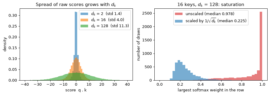
Unscaled, the largest weight is close to 1 in most draws and the mean entropy is a tenth of the uniform value: the softmax is nearly a hard lookup, and its Jacobian, which carries every gradient to \mathbf{W}_Q and \mathbf{W}_K, is nearly zero. Scaled, the rows are broad.
Step 10: multi-head shapes
The text of Section 4 follows a tensor of shape (B, T, d) through the multi-head
computation. Here is the same path with B = 2, T = 16, d = 256 and h = 8 heads of width
d_k = 32. The projection produces (B, T, d); view splits the last axis into heads;
transpose(1, 2) moves the head axis next to the batch axis, so that every matrix product acts on
the last two axes (T, d_k). At the end the heads are merged by transposing back and reshaping.
The result is compared with SDPA on the same projected tensors.
B, T, d, h = 2, 16, 256, 8
dk = d // h
x = torch.randn(B, T, d)
wq, wk, wv = (nn.Linear(d, d, bias=False) for _ in range(3))

q = wq(x).view(B, T, h, dk)
print("after the projection and view:", tuple(q.shape))
q = q.transpose(1, 2)
k = wk(x).view(B, T, h, dk).transpose(1, 2)
v = wv(x).view(B, T, h, dk).transpose(1, 2)
print("after transpose(1, 2):        ", tuple(q.shape))

scores = q @ k.transpose(-2, -1) / dk ** 0.5
print("scores:                       ", tuple(scores.shape))
causal_mask = torch.tril(torch.ones(T, T, dtype=torch.bool))
weights = scores.masked_fill(~causal_mask, float("-inf")).softmax(dim=-1)
per_head = weights @ v
print("per-head output:              ", tuple(per_head.shape))
merged = per_head.transpose(1, 2).reshape(B, T, d)
print("merged:                       ", tuple(merged.shape))

fused = F.scaled_dot_product_attention(q, k, v, is_causal=True)
print(f"max |explicit - fused| = {(per_head - fused).abs().max().item():.1e}")
after the projection and view: (2, 16, 8, 32)
after transpose(1, 2):         (2, 8, 16, 32)
scores:                        (2, 8, 16, 16)
per-head output:               (2, 8, 16, 32)
merged:                        (2, 16, 256)
max |explicit - fused| = 2.4e-07
The explicit softmax and the fused kernel agree to float32 rounding, about 10^{-7}. That is a
different precision from the 10^{-16} of the earlier steps, which is why those steps use
float64.
What you should see
- The NumPy and PyTorch outputs agree to better than 10^{-16} in
float64. The hand calculation, the formula and the fused kernel are one computation. - Every output row is a convex combination of the value rows it may see. With the mask, row 1 is exactly \mathbf{v}_1 whatever \mathbf{Q} and \mathbf{K} are.
- Removing the scale sharpens every row. Row 3’s largest weight rises from 0.503 to 0.576. At d_k = 128 the unscaled softmax is close to one-hot in most draws, so its Jacobian, and the gradient reaching \mathbf{W}_Q and \mathbf{W}_K, nearly vanish.
- The gradient with respect to the row-3 scores sums to zero, and only \mathbf{q}_3, the keys and the second column of \mathbf{V} receive gradient from \mathcal{L} = o_{3,2}.
Try this
- Multiply
Qby 10 and rerun Step 2. Row 3 approaches (0, 0, 1) and its output approaches \mathbf{v}_3 = (3, 3): the hard-lookup limit of Section 1. What happens to the Jacobian of Step 6? - Mask every key of one query (a fully padded row) and observe the result of your NumPy
softmax, which subtracts -\infty from -\infty, and of SDPA. Then write a guard that returns zeros for such a row. - Write multi-head attention with an explicit Python loop over the heads and check it against the batched version of Step 10 to 10^{-6}.
Lab 2 — RoPE, numerically
Goal. Implement rotary position embedding and test its relative-position property. Then deliberately break that property, compare real and complex implementations, and measure how frequencies and position interpolation change the scores. All inputs are synthetic; no download is needed. The last digits of the outputs may differ by machine.
Step 1: rotate adjacent pairs
Each row of x is a vector at the corresponding position. The final dimension must be
even: the rotation acts on pairs. A common offset applied to both query and key cancels
in their dot product, as derived in Section 6.
import numpy as np
import matplotlib.pyplot as plt
import torch

np.random.seed(0)
torch.manual_seed(0)
rng = np.random.default_rng(0)
np.set_printoptions(precision=3, suppress=True)


def rope_np(x, positions, base=10000.0):
    width = x.shape[-1]
    assert width % 2 == 0
    frequencies = base ** (-np.arange(0, width, 2) / width)
    angles = np.asarray(positions)[..., None] * frequencies
    first, second = x[..., 0::2], x[..., 1::2]
    result = np.empty_like(x)
    result[..., 0::2] = first * np.cos(angles) - second * np.sin(angles)
    result[..., 1::2] = first * np.sin(angles) + second * np.cos(angles)
    return result


q, k = np.array([[1., 0.]]), np.array([[0., 1.]])
for t, s in ((3, 1), (7, 5), (1, 3), (5, 5)):
    score = (rope_np(q, [t]) * rope_np(k, [s])).sum()
    print(f"positions ({t}, {s}): score {score:.3f}")
positions (3, 1): score 0.909
positions (7, 5): score 0.909
positions (1, 3): score -0.909
positions (5, 5): score 0.000
Step 2: test every diagonal
Use the same content vector at every position so that only position changes. A matrix constant along its diagonals is Toeplitz. Its diagonal offset is the relative position. This property does not say that scores in a real sentence are Toeplitz: content there varies.
positions = np.arange(64)
q = np.broadcast_to(rng.normal(size=64), (64, 64)).copy()
k = np.broadcast_to(rng.normal(size=64), (64, 64)).copy()
qr, kr = rope_np(q, positions), rope_np(k, positions)
scores = qr @ kr.T


def diagonal_deviation(matrix):
    return max(np.abs(np.diag(matrix, offset) -
                      np.diag(matrix, offset).mean()).max()
               for offset in range(1 - len(matrix), len(matrix)))


print(f"both rotated: diagonal deviation {diagonal_deviation(scores):.1e}")
norm_error = np.abs(np.linalg.norm(qr, axis=1) - np.linalg.norm(q, axis=1))
print(f"maximum norm change: {norm_error.max():.1e}")
broken = qr @ k.T
print(f"query only: diagonal deviation {diagonal_deviation(broken):.3f}")
assert diagonal_deviation(scores) < 1e-11
assert norm_error.max() < 1e-11
both rotated: diagonal deviation 2.1e-14
maximum norm change: 8.9e-16
query only: diagonal deviation 10.936
Rotating only the query leaves an absolute-position dependence. The code still runs and the shapes still match, which makes this a useful diagnostic for a misplaced RoPE call.
Step 3: real rotations against complex multiplication
The two real coordinates are the real and imaginary parts of one complex number. Multiplication by a unit complex number performs the same rotation. This tests the pairing convention as well as the signs. Other checkpoints can pair the first half of a head with the second half; they need a corresponding permutation of projection weights.
def rope(x, base=10000.0):
    B, h, T, dk = x.shape
    theta = base ** (-torch.arange(0, dk, 2, device=x.device) / dk)
    ang = torch.arange(T, device=x.device)[:, None] * theta[None, :]
    cos, sin = ang.cos()[None, None], ang.sin()[None, None]
    x1, x2 = x[..., 0::2], x[..., 1::2]
    return torch.stack([x1 * cos - x2 * sin, x1 * sin + x2 * cos],
                       dim=-1).flatten(-2)


x = torch.randn(2, 4, 32, 64)
theta = 10000.0 ** (-torch.arange(0, 64, 2) / 64)
angle = torch.arange(32)[:, None] * theta[None, :]
complex_x = torch.view_as_complex(x.reshape(2, 4, 32, 32, 2))
phase = torch.polar(torch.ones_like(angle), angle)
complex_result = torch.view_as_real(complex_x * phase).flatten(-2)
print(f"real versus complex: {(rope(x) - complex_result).abs().max():.1e}")
assert torch.allclose(rope(x), complex_result, atol=1e-6)
qt = torch.tensor(q[0], dtype=torch.float32).expand(1, 1, 256, 64)
kt = torch.tensor(k[0], dtype=torch.float32).expand(1, 1, 256, 64)
float_scores = (rope(qt) @ rope(kt).transpose(-1, -2))[0, 0].numpy()
print(f"float32, 256 positions: {diagonal_deviation(float_scores):.1e}")
real versus complex: 4.8e-07
float32, 256 positions: 4.4e-05
The float32 error grows with position because forming a larger angle loses more absolute precision. It is a numerical error, rather than a failure of the relative-position identity.
Step 4: wavelengths and oscillations
For aligned all-one vectors of width 128, the normalised dot product is the mean of the cosines of the 64 rotation angles. Individual frequencies oscillate; their sum has no guarantee of monotonic decay. The plot is an illustrative positional kernel, rather than a measurement of a trained head’s attention weights.
offsets = np.arange(1, 16385)
fig, ax = plt.subplots(figsize=(8, 4))
for base in (10000.0, 500000.0):
    frequencies = base ** (-np.arange(0, 128, 2) / 128)
    wavelengths = 2 * np.pi / frequencies
    correlation = np.cos(offsets[:, None] * frequencies).mean(axis=1)
    print(f"base {base:.0f}: wavelengths {wavelengths[0]:.2f} to "
          f"{wavelengths[-1]:.0f}; above 4096: {(wavelengths > 4096).sum()}/64")
    if base == 10000:
        for offset in (1, 16, 128, 1024, 4096):
            print(f"  offset {offset:5d}: {correlation[offset - 1]:.3f}")
    ax.plot(offsets, correlation, label=f"base {base:.0f}", alpha=0.8)
ax.set_xscale("log")
ax.set_xlabel("relative position (tokens)")
ax.set_ylabel("dot product / dot product at zero offset")
ax.set_title("RoPE positional kernel for aligned all-one vectors")
ax.legend()
plt.tight_layout()
plt.show()
base 10000: wavelengths 6.28 to 54410; above 4096: 18/64
  offset     1: 0.970
  offset    16: 0.620
  offset   128: 0.333
  offset  1024: 0.204
  offset  4096: -0.053
base 500000: wavelengths 6.28 to 2559196; above 4096: 32/64
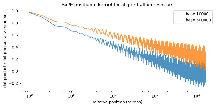
Step 5: interpolation and ALiBi
Dividing positions by four maps 256 positions onto approximately the angular range of 64 original positions. At positions divisible by four the score matrix exactly matches the original one. This equality alone does not prove that a trained model works at the longer length: intermediate spacings and the distribution of competing keys have changed.
long_positions = np.arange(256) / 4
long_q = np.broadcast_to(q[0], (256, 64))
long_k = np.broadcast_to(k[0], (256, 64))
interpolated = rope_np(long_q, long_positions) @ rope_np(long_k, long_positions).T
print(f"interpolated submatrix error: {np.abs(interpolated[::4, ::4] - scores).max():.1e}")
assert np.allclose(interpolated[::4, ::4], scores, atol=1e-11)
slopes = 2.0 ** (-np.arange(1, 9))
distance = np.maximum(0, np.arange(6)[:, None] - np.arange(6)[None, :])
bias = -slopes[:, None, None] * distance
print("ALiBi slopes:", slopes)
print("first head's bias:")
print(bias[0])
interpolated submatrix error: 0.0e+00
ALiBi slopes: [0.5   0.25  0.125 0.062 0.031 0.016 0.008 0.004]
first head's bias:
[[-0.  -0.  -0.  -0.  -0.  -0. ]
 [-0.5 -0.  -0.  -0.  -0.  -0. ]
 [-1.  -0.5 -0.  -0.  -0.  -0. ]
 [-1.5 -1.  -0.5 -0.  -0.  -0. ]
 [-2.  -1.5 -1.  -0.5 -0.  -0. ]
 [-2.5 -2.  -1.5 -1.  -0.5 -0. ]]
The zero entries above the diagonal are not permission to read future tokens. Apply a separate causal mask. These geometric slopes are for eight heads; arbitrary head counts need the slope construction used by the intended implementation.
What you should see
Rotating both vectors preserves norms and diagonal scores to rounding error. Rotating only one breaks the diagonal property. A larger base gives more slow pairs, and dividing positions by four preserves the original scores on the corresponding submatrix.
Try this
- Compute the NTK-aware base
10000 * 4 ** (128 / 126)and compare wavelengths. - Pair coordinate
iwithi + 32instead of adjacent coordinates. Check Toeplitzness, then show that the scores differ for the same unpermuted vectors. - Add rotations to the three-token example and shift all positions by seven. Verify that every output is unchanged when both queries and keys receive the shift.
Lab 3 — Online softmax and tiled attention
Goal. Compute exact attention without materialising its entire score matrix. Implement the running softmax normaliser, trace the three-token example, and compare tiled attention with a dense reference. This NumPy experiment measures storage and numerical agreement; its CPU timing does not predict a GPU kernel’s speed.
Step 1: avoid overflow
import time
import numpy as np

np.random.seed(0)
rng = np.random.default_rng(0)
np.set_printoptions(precision=3, suppress=True)


def safe_softmax(scores):
    weights = np.exp(scores - scores.max(axis=-1, keepdims=True))
    return weights / weights.sum(axis=-1, keepdims=True)


large = np.array([1000., 1001., 1002.])
with np.errstate(over="ignore", invalid="ignore"):
    naive = np.exp(large) / np.exp(large).sum()
print("naive:", naive)
print("safe: ", safe_softmax(large))
naive: [nan nan nan]
safe:  [0.09  0.245 0.665]
Subtracting the maximum cancels between numerator and denominator. The largest exponential becomes one, and none can overflow.
Step 2: stream the normaliser
The current maximum defines the scale of the accumulated sum. When a later score
raises that maximum, multiply the old sum by exp(old_max - new_max) before adding
the new term. A second pass is needed to emit every probability; attention avoids that
pass by accumulating the weighted values directly.
def online_softmax_stats(scores):
    maximum, normaliser = -np.inf, 0.0
    for score in scores:
        new_maximum = max(maximum, score)
        normaliser = (normaliser * np.exp(maximum - new_maximum)
                      + np.exp(score - new_maximum))
        maximum = new_maximum
    return maximum, normaliser


scores = rng.normal(0, 5, 10000)
maximum, normaliser = online_softmax_stats(scores)
online = np.exp(scores - maximum) / normaliser
print(f"online versus safe: {np.abs(online - safe_softmax(scores)).max():.1e}")
assert np.allclose(online, safe_softmax(scores), atol=1e-14)
online versus safe: 8.9e-16
Step 3: trace the output accumulator
The accumulator holds an unnormalised weighted sum of value vectors. Its scale must change with the normaliser’s scale; rescaling just one of them produces a wrong answer.
Q = np.array([[1., 0.], [0., 1.], [1., 1.]])
K = Q.copy()
V = np.array([[1., 0.], [0., 2.], [3., 3.]])
row = Q[2] @ K.T / np.sqrt(2)
maximum, normaliser, accumulator = -np.inf, 0., np.zeros(2)
for start in (0, 2):
    block = row[start:start + 2]
    new_maximum = max(maximum, block.max())
    rescale = np.exp(maximum - new_maximum)
    weights = np.exp(block - new_maximum)
    accumulator = accumulator * rescale + weights @ V[start:start + 2]
    normaliser = normaliser * rescale + weights.sum()
    maximum = new_maximum
    print(f"block {start // 2 + 1}: m={maximum:.3f}, rescale={rescale:.3f}, "
          f"l={normaliser:.3f}, a={accumulator}")
print("output:", accumulator / normaliser)
block 1: m=0.707, rescale=0.000, l=2.000, a=[1. 2.]
block 2: m=1.414, rescale=0.493, l=1.986, a=[3.493 3.986]
output: [1.759 2.007]
Step 4: tile queries and keys
Each query row keeps its own maximum, normaliser and accumulator. Skip key blocks entirely in the future, and mask future entries inside a diagonal block. The code supports unequal tile dimensions: some rows in such a tile can have no visible keys. For those rows, a finite fallback maximum keeps their zero contribution free of NaNs.
def tiled_attention(Q, K, V, Br=64, Bc=64, causal=True):
    assert Br > 0 and Bc > 0
    assert Q.shape == K.shape and len(Q) == len(V)
    T, width = Q.shape
    output = np.empty((T, V.shape[1]), dtype=Q.dtype)
    tiles, largest = 0, 0
    for row_start in range(0, T, Br):
        query = Q[row_start:row_start + Br]
        rows = row_start + np.arange(len(query))
        maximum = np.full(len(query), -np.inf, dtype=Q.dtype)
        normaliser = np.zeros(len(query), dtype=Q.dtype)
        acc = np.zeros((len(query), V.shape[1]), dtype=Q.dtype)
        key_stop = min(T, row_start + Br) if causal else T
        for key_start in range(0, key_stop, Bc):
            key = K[key_start:key_start + Bc]
            scores = query @ key.T / np.sqrt(width)
            if causal:
                columns = key_start + np.arange(len(key))
                scores = np.where(columns[None, :] <= rows[:, None], scores, -np.inf)
            new_max = np.maximum(maximum, scores.max(axis=1))
            finite_max = np.where(np.isfinite(new_max), new_max, 0)
            rescale = np.exp(maximum - finite_max)
            weights = np.exp(scores - finite_max[:, None])
            acc = acc * rescale[:, None] + weights @ V[key_start:key_start + Bc]
            normaliser = normaliser * rescale + weights.sum(axis=1)
            maximum = new_max
            tiles += 1
            largest = max(largest, scores.nbytes)
        output[row_start:row_start + Br] = acc / normaliser[:, None]
    return output, tiles, largest


def dense_attention(Q, K, V, causal=True):
    scores = Q @ K.T / np.sqrt(Q.shape[1])
    if causal:
        scores = np.where(np.tri(len(Q), dtype=bool), scores, -np.inf)
    return safe_softmax(scores) @ V


print("three-token tiled output:")
print(tiled_attention(Q, K, V, Br=1, Bc=2)[0])
Q, K, V = (rng.normal(size=(1024, 64)) for _ in range(3))
for causal in (True, False):
    reference = dense_attention(Q, K, V, causal)
    result, tiles, largest = tiled_attention(Q, K, V, causal=causal)
    print(f"causal={causal}: float64 error {np.abs(result - reference).max():.1e}, "
          f"tiles {tiles}/256, largest scores {largest // 1024} KiB")
    assert np.allclose(result, reference, atol=1e-12)
    float_inputs = [a.astype(np.float32) for a in (Q, K, V)]
    float_result = tiled_attention(*float_inputs, causal=causal)[0]
    float_dense = dense_attention(*float_inputs, causal=causal)
    print(f"  float32 tiled error {np.abs(float_result - reference).max():.1e}, "
          f"dense error {np.abs(float_dense - reference).max():.1e}")
    assert np.allclose(float_result, reference, atol=2e-6)
print(f"dense scores: {1024 ** 2 * 8 // 1024 ** 2} MiB")
for Br, Bc in ((32, 128), (37, 53)):
    result = tiled_attention(Q, K, V, Br=Br, Bc=Bc)[0]
    assert np.allclose(result, dense_attention(Q, K, V), atol=1e-12)
print("unequal and non-dividing tiles: passed")
three-token tiled output:
[[1.    0.   ]
 [0.33  1.34 ]
 [1.759 2.007]]
causal=True: float64 error 5.6e-16, tiles 136/256, largest scores 32 KiB
  float32 tiled error 3.4e-07, dense error 3.3e-07
causal=False: float64 error 1.7e-16, tiles 256/256, largest scores 32 KiB
  float32 tiled error 1.7e-07, dense error 1.7e-07
dense scores: 8 MiB
unequal and non-dividing tiles: passed
The largest score tile is 32 KiB, compared with 8 MiB for the dense scores. This is score storage only: the tiled code also holds weights for a tile, accumulators and input/output arrays. It is an educational forward implementation, without a custom backward pass or GPU memory hierarchy.
Step 5: time the CPU implementations
for name, function in (("dense", dense_attention), ("tiled", tiled_attention)):
    started = time.perf_counter()
    function(Q, K, V)
    print(f"{name}: {time.perf_counter() - started:.3f} seconds (CPU NumPy)")
dense: 0.012 seconds (CPU NumPy)
tiled: 0.008 seconds (CPU NumPy)
These one-run times depend on BLAS, thread count and other processes. On a GPU the point of FlashAttention is to avoid writing and rereading the large score and weight matrices in HBM. Python loops on a CPU do not reproduce that performance comparison.
What you should see
Online, dense and tiled results agree to rounding error. Causal 64-by-64 tiling computes 136 of 256 tiles. Repartitioning into unequal or incomplete tiles preserves the answer.
Try this
- Remove accumulator rescaling. Use the three-token example to identify the first block where the result becomes wrong.
- Store each row’s log-sum-exp and recompute probability tiles in a backward pass. Compare gradients with PyTorch autograd at sequence length 128.
- Count score storage at lengths 512, 1024 and 2048 while keeping tile sizes fixed. Separate input/output storage from intermediate score storage.
Lab 4 — A parameter and FLOP counter for Llama-style models
Goal. Write a counter that reads a decoder’s configuration (vocabulary size, width, depth,
query heads, key-value heads, feed-forward width, tying, biases) and returns its parameter count,
its FLOPs per token under the convention of Section 11, and its KV-cache size per token.
Then check the counter three ways: against PyTorch, by building the module’s own Decoder;
against the sizes published for five open models, from GPT-2 small to Llama-3-8B; and, if
Hugging Face transformers is installed, against the reference implementations of those five
models, built on PyTorch’s meta device so that an eight-billion-parameter model costs neither
memory nor a download. With the counter in hand you will see why the 12Ld^2 rule is within 1%
for one model and 55% out for another, how much of a small model is embedding table, what
grouped-query attention does to the cache, and at what context length attention stops being a
rounding error in the FLOP count. The configurations are typed in from each model’s
config.json; nothing is downloaded and the lab runs in seconds.
Step 1 — Set up
Counting needs no randomness, but every lab in the series fixes its seeds first, so that any tensor it creates (here, the decoders built in Step 3) is the same on every run.
from dataclasses import dataclass

import matplotlib.pyplot as plt
import numpy as np
import torch
import torch.nn as nn
import torch.nn.functional as F

np.random.seed(0)
torch.manual_seed(0)
Step 2 — Describe a model, then count it
A decoder-only transformer is pinned down by a handful of numbers and switches:
- the vocabulary size V and the width d of the residual stream;
- the number of layers L, each with h query heads of width d_{\text{head}} = d/h and n_{kv} key-value heads: n_{kv} = h is multi-head attention, 1 < n_{kv} < h is grouped-query attention and n_{kv} = 1 is multi-query attention (Section 9);
- the feed-forward width d_{\text{ff}}, and whether the feed-forward network is SwiGLU (three matrices) or a plain two-matrix MLP (Section 5);
- whether the output projection is tied to the input embedding;
- which linear layers carry biases, whether positions come from a learned table (GPT-2) or from RoPE (no parameters at all), and whether each norm is LayerNorm (a gain and a bias, 2d numbers) or RMSNorm (a gain only, d numbers).
The counter adds the pieces up block by block, exactly as Section 11 does. Each layer holds
and the model adds, once, a token table of Vd numbers, a second Vd if the output projection is untied, T_{\max} d for a learned position table, and a final norm. Since h d_{\text{head}} = d in every model here, the attention line is 2d^2 + 2d\,n_{kv} d_{\text{head}}, which is 4d^2 for multi-head attention and less under grouping.
The counter also returns N_{\text{matmul}}, the parameters that take part in a matrix multiply for every token. It is N_{\text{total}} minus the lookup tables, which are an untied input embedding and a learned position table: reading row i of a table costs no arithmetic. A tied matrix stays in N_{\text{matmul}}, because it is still used once per token, as the output projection. The dictionary keeps per-layer and whole-model figures apart, because the per-layer ones are what you compare with a paper’s description of one block.
@dataclass
class Cfg:
    name: str
    V: int                   # vocabulary size
    d: int                   # width of the residual stream
    L: int                   # number of layers (blocks)
    h: int                   # query heads
    n_kv: int                # key-value heads: h is multi-head, 1 is multi-query
    d_ff: int                # inner width of the feed-forward network
    tied: bool               # does the output projection reuse the input embedding?
    glu: bool = True         # SwiGLU (three matrices) or a plain two-matrix MLP
    bias: str = "none"       # "none", "qkv" (on W_Q, W_K, W_V only) or "all"
    learned_pos: int = 0     # rows of a learned position table (0 with RoPE)
    norm_bias: bool = False  # LayerNorm has a gain and a bias; RMSNorm a gain only
    published: str = "-"     # the size its authors quote


def count(cfg):
    """Parameters of a decoder-only transformer, itemised as in Section 11."""
    d_head = cfg.d // cfg.h
    q_width = cfg.h * d_head        # all query heads side by side (equals d here)
    kv_width = cfg.n_kv * d_head    # narrower than d under GQA and MQA

    # Attention: W_Q is d x q_width, W_K and W_V are d x kv_width, W_O is q_width x d.
    attention = cfg.d * q_width + 2 * cfg.d * kv_width + q_width * cfg.d
    if cfg.bias in ("qkv", "all"):
        attention += q_width + 2 * kv_width     # one bias per output unit
    if cfg.bias == "all":
        attention += cfg.d                      # and one on W_O

    # Feed-forward: W_1 and W_3 (d x d_ff) and W_2 (d_ff x d), or W_1 and W_2 only.
    mlp = (3 if cfg.glu else 2) * cfg.d * cfg.d_ff
    if cfg.bias == "all":
        mlp += (2 if cfg.glu else 1) * cfg.d_ff + cfg.d

    # Two norms per layer (before attention, before the FFN) and one at the end.
    one_norm = 2 * cfg.d if cfg.norm_bias else cfg.d
    per_layer = attention + mlp + 2 * one_norm

    token_table = cfg.V * cfg.d
    embeddings = token_table * (1 if cfg.tied else 2) + cfg.learned_pos * cfg.d
    total = embeddings + cfg.L * per_layer + one_norm

    # A lookup is not a matrix multiply: an untied input embedding and a position
    # table cost no FLOPs. A tied table stays in, because it is used once per
    # token as the output projection.
    lookups = (0 if cfg.tied else token_table) + cfg.learned_pos * cfg.d
    return {
        "attention_per_layer": attention,
        "mlp_per_layer": mlp,
        "norms_per_layer": 2 * one_norm,
        "embeddings": embeddings,
        "attention": cfg.L * attention,
        "mlp": cfg.L * mlp,
        "norms": cfg.L * 2 * one_norm + one_norm,
        "total": total,
        "n_matmul": total - lookups,
    }


llama2 = Cfg("Llama-2-7B", V=32000, d=4096, L=32, h=32, n_kv=32, d_ff=11008,
             tied=False, published="6.7B")
c = count(llama2)
layer = c["attention_per_layer"] + c["mlp_per_layer"] + c["norms_per_layer"]
print(f"attention per layer   {c['attention_per_layer']:>15,}")
print(f"FFN per layer         {c['mlp_per_layer']:>15,}")
print(f"norms per layer       {c['norms_per_layer']:>15,}")
print(f"one layer             {layer:>15,}")
print(f"{llama2.L} layers             {llama2.L * layer:>15,}")
print(f"embeddings (untied)   {c['embeddings']:>15,}")
print(f"final norm            {llama2.d:>15,}")
print(f"N_total               {c['total']:>15,}")
print(f"N_matmul              {c['n_matmul']:>15,}")
attention per layer        67,108,864
FFN per layer             135,266,304
norms per layer                 8,192
one layer                 202,383,360
32 layers               6,476,267,520
embeddings (untied)       262,144,000
final norm                      4,096
N_total                 6,738,415,616
N_matmul                6,607,343,616
Every line is a product you can redo by hand. The attention layer is four 4096 \times 4096 matrices, 4 \times 16{,}777{,}216 = 67{,}108{,}864. The SwiGLU network is three 4096 \times 11{,}008 matrices, 135{,}266{,}304, a little more than the 8d^2 = 134{,}217{,}728 of the rule because 11{,}008 is \tfrac{8}{3}d = 10{,}922.7 rounded up to a multiple of 256. The two RMSNorm gains add 2 \times 4{,}096 = 8{,}192. Thirty-two layers, two untied 32{,}000 \times 4{,}096 tables and a final norm make 6{,}738{,}415{,}616, the 6.7B of the Llama 2 paper. Removing the input table, which is a lookup, leaves N_{\text{matmul}} = 6{,}607{,}343{,}616: the number that the FLOP count of Step 7 multiplies.
Step 3 — Check the counter against PyTorch
A formula is only as good as its check, and the surest check is a model built in code: PyTorch
knows every tensor it allocated. The block below is the Decoder of Section 12,
reformatted to 88-character lines but otherwise the same, including the initialisation line
and the causal switch that Lab 5 uses. Counting does not depend on either.
Build it twice, at the module’s default size (vocabulary 4,096, d = 256, four layers, eight
query heads, two KV heads) and at the size Lab 5 trains (vocabulary 46, d = 128, four layers,
four query heads, two KV heads), and compare the counter with the sum of the tensors. One
subtlety decides the answer. The output projection and the input embedding are a single tensor
(self.head.weight = self.emb.weight), and model.parameters() yields each tensor once, so the
shared matrix is counted once. A script that walks the modules and adds up every weight it meets
counts it twice; the last line shows the number such a script would report.
def rope(x, base=10000.0):
    """x: (B, h, T, dk). Rotate pairs of dims by position-dependent angles."""
    B, h, T, dk = x.shape
    theta = base ** (-torch.arange(0, dk, 2, device=x.device) / dk)   # (dk/2,)
    ang = torch.arange(T, device=x.device)[:, None] * theta[None, :]   # (T, dk/2)
    cos, sin = ang.cos()[None, None], ang.sin()[None, None]
    x1, x2 = x[..., 0::2], x[..., 1::2]
    return torch.stack([x1 * cos - x2 * sin, x1 * sin + x2 * cos], dim=-1).flatten(-2)


class Attention(nn.Module):
    def __init__(self, d, n_heads, n_kv_heads, causal=True):
        super().__init__()
        self.h, self.kv, self.dk = n_heads, n_kv_heads, d // n_heads
        self.causal = causal
        self.wq = nn.Linear(d, d, bias=False)
        self.wk = nn.Linear(d, n_kv_heads * self.dk, bias=False)
        self.wv = nn.Linear(d, n_kv_heads * self.dk, bias=False)
        self.wo = nn.Linear(d, d, bias=False)

    def forward(self, x):
        B, T, d = x.shape
        q = self.wq(x).view(B, T, self.h, self.dk).transpose(1, 2)    # (B, h, T, dk)
        k = self.wk(x).view(B, T, self.kv, self.dk).transpose(1, 2)
        v = self.wv(x).view(B, T, self.kv, self.dk).transpose(1, 2)
        q, k = rope(q), rope(k)
        k = k.repeat_interleave(self.h // self.kv, dim=1)    # grouped-query: share KV
        v = v.repeat_interleave(self.h // self.kv, dim=1)
        y = F.scaled_dot_product_attention(q, k, v, is_causal=self.causal)
        return self.wo(y.transpose(1, 2).reshape(B, T, d))


class Block(nn.Module):
    def __init__(self, d, n_heads, n_kv_heads, d_ff, causal=True):
        super().__init__()
        self.n1, self.n2 = nn.RMSNorm(d), nn.RMSNorm(d)
        self.attn = Attention(d, n_heads, n_kv_heads, causal)
        self.w1 = nn.Linear(d, d_ff, bias=False)
        self.w3 = nn.Linear(d, d_ff, bias=False)
        self.w2 = nn.Linear(d_ff, d, bias=False)

    def forward(self, x):
        x = x + self.attn(self.n1(x))                           # pre-norm residual
        h = self.n2(x)
        return x + self.w2(F.silu(self.w1(h)) * self.w3(h))    # SwiGLU feed-forward


class Decoder(nn.Module):
    def __init__(self, vocab, d=256, layers=4, n_heads=8, n_kv_heads=2, d_ff=None,
                 causal=True):
        super().__init__()
        d_ff = d_ff or int(8 * d / 3)
        self.emb = nn.Embedding(vocab, d)
        self.blocks = nn.ModuleList(Block(d, n_heads, n_kv_heads, d_ff, causal)
                                    for _ in range(layers))
        self.norm = nn.RMSNorm(d)
        self.head = nn.Linear(d, vocab, bias=False)
        self.head.weight = self.emb.weight                          # tied embeddings
        nn.init.normal_(self.emb.weight, std=0.02)    # keeps step-0 logits small

    def forward(self, tokens):                                  # tokens: (B, T) ints
        x = self.emb(tokens)
        for b in self.blocks:
            x = b(x)
        return self.head(self.norm(x))                          # logits: (B, T, vocab)


tiny = Cfg("tiny decoder", V=4096, d=256, L=4, h=8, n_kv=2, d_ff=int(8 * 256 / 3),
           tied=True)
lab5 = Cfg("Lab 5 decoder", V=46, d=128, L=4, h=4, n_kv=2, d_ff=int(8 * 128 / 3),
           tied=True)
for cfg in (tiny, lab5):
    model = Decoder(vocab=cfg.V, d=cfg.d, layers=cfg.L, n_heads=cfg.h,
                    n_kv_heads=cfg.n_kv)
    in_torch = sum(p.numel() for p in model.parameters())   # shared tensor: once
    print(f"{cfg.name:<14} d_ff {cfg.d_ff:>3}   counter {count(cfg)['total']:>10,}"
          f"   PyTorch {in_torch:>10,}")

model = Decoder(vocab=4096)
print("head and embedding are one tensor:", model.head.weight is model.emb.weight)
twice = sum(p.numel() for _, p in model.named_parameters(remove_duplicate=False))
print(f"counting the shared matrix twice would give {twice:,}")
tiny decoder   d_ff 682   counter  3,801,344   PyTorch  3,801,344
Lab 5 decoder  d_ff 341   counter    727,424   PyTorch    727,424
head and embedding are one tensor: True
counting the shared matrix twice would give 4,849,920
The counter and PyTorch agree to the parameter at both sizes: 3,801,344 is the “about 3.8M”
that the decoder’s code prints in Section 12, and 727,424 is the model Lab 5 trains. Note
d_ff: \tfrac{8}{3} \times 256 = 682.7 and \tfrac{8}{3} \times 128 = 341.3, and int
truncates both. Counting the shared matrix twice adds the 4{,}096 \times 256 = 1{,}048{,}576
numbers of the table again and overstates the model by 28%, a mistake that is easy to make when
parameters are counted from a state_dict, which lists the shared tensor under both of its names.
Exercise 12 asks you to itemise the 3,801,344 by hand; do it before Step 4 if you have
not, and compare each part with the dictionary that count(tiny) returns.
Step 4 — Five published models against the rule
Now the published models. The configurations below are copied from each model’s config.json,
and each has a feature that the 12Ld^2 rule does not know about:
- GPT-2 small (2019): multi-head attention, a GELU MLP of width 4d, biases on every linear layer, LayerNorm with a bias, a learned table of 1,024 positions, tied embeddings.
- SmolLM2-135M: nine query heads sharing three KV heads, a SwiGLU network of width 1{,}536 = \tfrac{8}{3}d, tied embeddings.
- Qwen2.5-0.5B: fourteen query heads sharing two KV heads, biases on \mathbf{W}_Q, \mathbf{W}_K and \mathbf{W}_V only, an unusually wide SwiGLU network (4{,}864 \approx 5.4d) and a 151,936-token vocabulary, tied.
- Llama-2-7B: the configuration of Step 2.
- Llama-3-8B: 32 query heads sharing 8 KV heads, a SwiGLU width of 14{,}336 = 3.5d, and a 128,256-token vocabulary, untied.
The block prints, for each model, the exact count, the rule 12Ld^2, the ratio of the non-embedding parameters to the rule, the share of the parameters that sits in embeddings (token tables, plus the position table for GPT-2) and the size the authors quote. A second table expresses one layer in units of d^2, which is the language in which the rule is wrong.
configs = [
    tiny,
    Cfg("GPT-2 small", V=50257, d=768, L=12, h=12, n_kv=12, d_ff=3072, tied=True,
        glu=False, bias="all", learned_pos=1024, norm_bias=True, published="124M"),
    Cfg("SmolLM2-135M", V=49152, d=576, L=30, h=9, n_kv=3, d_ff=1536, tied=True,
        published="135M"),
    Cfg("Qwen2.5-0.5B", V=151936, d=896, L=24, h=14, n_kv=2, d_ff=4864, tied=True,
        bias="qkv", published="0.49B"),
    llama2,
    Cfg("Llama-3-8B", V=128256, d=4096, L=32, h=32, n_kv=8, d_ff=14336, tied=False,
        published="8B"),
]

print(f"{'model':<16}{'N_total':>15}{'12Ld^2':>15}{'ratio':>7}{'emb':>7}"
      f"{'published':>11}")
for cfg in configs:
    c = count(cfg)
    rule = 12 * cfg.L * cfg.d ** 2
    non_embedding = c["total"] - c["embeddings"]
    print(f"{cfg.name:<16}{c['total']:>15,}{rule:>15,}{non_embedding / rule:>7.3f}"
          f"{c['embeddings'] / c['total']:>7.1%}{cfg.published:>11}")

print("\none layer in units of d^2 (the rule assumes 4 + 8 = 12)")
for cfg in configs:
    c = count(cfg)
    d2 = cfg.d ** 2
    print(f"{cfg.name:<16} attention {c['attention_per_layer'] / d2:5.2f}"
          f"   FFN {c['mlp_per_layer'] / d2:5.2f}"
          f"   layer {(c['attention_per_layer'] + c['mlp_per_layer']) / d2:5.2f}")
model                   N_total         12Ld^2  ratio    emb  published
tiny decoder          3,801,344      3,145,728  0.875  27.6%          -
GPT-2 small         124,439,808     84,934,656  1.001  31.6%       124M
SmolLM2-135M        134,515,008    119,439,360  0.889  21.0%       135M
Qwen2.5-0.5B        494,032,768    231,211,008  1.548  27.6%      0.49B
Llama-2-7B        6,738,415,616  6,442,450,944  1.005   3.9%       6.7B
Llama-3-8B        8,030,261,248  6,442,450,944  1.083  13.1%         8B

one layer in units of d^2 (the rule assumes 4 + 8 = 12)
tiny decoder     attention  2.50   FFN  7.99   layer 10.49
GPT-2 small      attention  4.01   FFN  8.01   layer 12.01
SmolLM2-135M     attention  2.67   FFN  8.00   layer 10.67
Qwen2.5-0.5B     attention  2.29   FFN 16.29   layer 18.57
Llama-2-7B       attention  4.00   FFN  8.06   layer 12.06
Llama-3-8B       attention  2.50   FFN 10.50   layer 13.00
Each count rounds to the size its authors quote, and each departure from the rule can be read off the second table. Under grouping, \mathbf{W}_K and \mathbf{W}_V map d to n_{kv} d_{\text{head}} = (n_{kv}/h)\,d dimensions, so attention costs 2d^2 + 2d^2 n_{kv}/h instead of 4d^2: 2 + 2/3 = 2.67 for SmolLM2 (three KV heads for nine), 2 + 2/7 = 2.29 for Qwen2.5 (two for fourteen) and 2 + 2/4 = 2.5 for Llama-3 and for the tiny decoder (two for eight). The feed-forward network costs 3 d_{\text{ff}}/d in units of d^2: exactly 8 when d_{\text{ff}} = \tfrac{8}{3}d (SmolLM2), 3 \times 3.5 = 10.5 for Llama-3 and 3 \times 5.43 = 16.29 for Qwen2.5, whose feed-forward network alone is larger than the rule’s whole layer. So the non-embedding count is 11% below the rule for SmolLM2-135M and 55% above it for Qwen2.5-0.5B, while for GPT-2 small and Llama-2-7B, the two models built the way the rule assumes, it is within 0.5% of it.
The embedding column tells the other half of the story. A vocabulary of 50,000 to 150,000 tokens times a width of 576 to 896 is tens of millions of parameters, so embeddings are a fifth to a third of every small model here; in Llama-2-7B the same kind of table is under 4%. Llama-3-8B climbs back to 13% because its vocabulary is four times Llama 2’s and its tables are untied. The lesson is the one Section 11 draws: count from the configuration, not from the rule, and quote the rule only for what it is, an estimate that holds for large multi-head models with d_{\text{ff}} \approx \tfrac{8}{3}d (SwiGLU) or 4d (GELU).
Step 5 — The KV cache per token
During generation every layer keeps the keys and values of every past token (Section 9), so the cache grows by
where the 2 counts K and V and a bf16 value takes 2 bytes. Query heads do not appear: only the n_{kv} key-value heads are stored. As in Section 9, sizes computed from tensor shapes are given in binary units (1 KiB = 1,024 B, 1 MiB = 2^{20} B, 1 GiB = 2^{30} B), and a size that Modules 07 to 10 quote in decimal gigabytes is given in both forms. The second half of the block holds the Llama-2-7B shape fixed and changes only n_{kv}, the comparison that Figure 6.15 draws, and sets the cache of one 4,096-token sequence beside the weights.
def kv_cache_bytes_per_token(cfg, bytes_per_value=2):
    """K and V of one token, in every layer and every KV head (bf16: 2 bytes)."""
    d_head = cfg.d // cfg.h
    return 2 * cfg.L * cfg.n_kv * d_head * bytes_per_value


print(f"{'model':<16}{'KV heads':>9}{'bytes/token':>13}{'KiB':>8}")
for cfg in configs:
    per_token = kv_cache_bytes_per_token(cfg)
    print(f"{cfg.name:<16}{cfg.n_kv:>9}{per_token:>13,}{per_token / 1024:>8.1f}")

seq_len = 4096
print(f"\none {seq_len:,}-token sequence at the Llama-2-7B shape, bf16")
for label, n_kv in (("multi-head, 32 KV heads", 32), ("grouped, 8 KV heads", 8),
                    ("multi-query, 1 KV head", 1)):
    shape = Cfg(label, V=32000, d=4096, L=32, h=32, n_kv=n_kv, d_ff=11008,
                tied=False)
    per_token = kv_cache_bytes_per_token(shape)
    per_sequence = per_token * seq_len
    print(f"{label:<24}{per_token:>9,} B/token {per_sequence / 2**20:>7,.0f} MiB"
          f"  ({per_sequence / 1e9:.3f} GB)")
weight_bytes = count(llama2)["total"] * 2
print(f"Llama-2-7B weights in bf16: {weight_bytes / 1e9:.1f} GB"
      f" ({weight_bytes / 2**30:.1f} GiB)")
model            KV heads  bytes/token     KiB
tiny decoder            2        1,024     1.0
GPT-2 small            12       36,864    36.0
SmolLM2-135M            3       23,040    22.5
Qwen2.5-0.5B            2       12,288    12.0
Llama-2-7B             32      524,288   512.0
Llama-3-8B              8      131,072   128.0

one 4,096-token sequence at the Llama-2-7B shape, bf16
multi-head, 32 KV heads   524,288 B/token   2,048 MiB  (2.147 GB)
grouped, 8 KV heads       131,072 B/token     512 MiB  (0.537 GB)
multi-query, 1 KV head     16,384 B/token      64 MiB  (0.067 GB)
Llama-2-7B weights in bf16: 13.5 GB (12.6 GiB)
The cache follows the KV heads, not the parameters. GPT-2 small keeps all twelve of its heads and caches three times as much per token as Qwen2.5-0.5B, a model four times its size whose fourteen query heads share two KV heads. At the Llama-2-7B shape one 4,096-token sequence needs 2,048 MiB = 2 GiB (2.15 GB) of cache, a sixth of the 12.6 GiB of weights, so about six such sequences in flight hold as much cache as the model holds weights; grouping eight KV heads (Llama-3-8B’s layout) cuts the cache four-fold to 512 MiB, and a single KV head eight-fold more, to 64 MiB. That ratio, cache per sequence against weights, is what decides how many requests a server can batch, and Module 10 builds its memory budget from exactly this formula.
Step 6 — Optional: the reference implementations, on the meta device
The published sizes are rounded, so they cannot confirm the last digit. The reference
implementations in Hugging Face transformers can, without downloading a single weight. On
PyTorch’s meta device a tensor has a shape and a dtype but no storage, so building a model
inside with torch.device("meta"): runs every constructor, registers every parameter and
allocates nothing: an eight-billion-parameter model is built in a fraction of a second in a few
kilobytes. The configuration classes take the same numbers as Cfg. GPT-2’s default
configuration is GPT-2 small, SmolLM2 and both Llamas use the Llama classes, and Qwen2.5 uses
the Qwen2 classes, which put biases on the query, key and value projections. If transformers
is not installed, the block says so and the lab carries on.
try:
    from transformers import (GPT2Config, GPT2LMHeadModel, LlamaConfig,
                              LlamaForCausalLM, Qwen2Config, Qwen2ForCausalLM)
    have_transformers = True
except ImportError:
    have_transformers = False
    print("transformers is not installed: skipping the cross-check")


def reference_model(cfg):
    """The Hugging Face implementation of a configuration (weights not allocated
    when built on the meta device)."""
    if cfg.name == "GPT-2 small":
        return GPT2LMHeadModel(GPT2Config())       # the defaults are GPT-2 small
    shape = dict(vocab_size=cfg.V, hidden_size=cfg.d, intermediate_size=cfg.d_ff,
                 num_hidden_layers=cfg.L, num_attention_heads=cfg.h,
                 num_key_value_heads=cfg.n_kv, tie_word_embeddings=cfg.tied)
    if cfg.bias == "qkv":
        return Qwen2ForCausalLM(Qwen2Config(**shape))
    return LlamaForCausalLM(LlamaConfig(**shape))


if have_transformers:
    for cfg in configs[1:]:
        with torch.device("meta"):         # shapes only: no memory is allocated
            reference = reference_model(cfg)
        n_reference = sum(p.numel() for p in reference.parameters())
        verdict = "same" if n_reference == count(cfg)["total"] else "DIFFERENT"
        print(f"{cfg.name:<14} transformers {n_reference:>15,}   counter "
              f"{count(cfg)['total']:>15,}   {verdict}")
GPT-2 small    transformers     124,439,808   counter     124,439,808   same
SmolLM2-135M   transformers     134,515,008   counter     134,515,008   same
Qwen2.5-0.5B   transformers     494,032,768   counter     494,032,768   same
Llama-2-7B     transformers   6,738,415,616   counter   6,738,415,616   same
Llama-3-8B     transformers   8,030,261,248   counter   8,030,261,248   same
All five agree to the parameter. The reference code was written by other people for other purposes, so the agreement checks every assumption the counter makes: where the biases are, that GPT-2’s position table and LayerNorm biases count, that the tied tables are shared and the untied ones are not.
Step 7 — Forward FLOPs per token
Section 11 fixed the convention: a product of an (m \times n) and an (n \times p) matrix costs 2mnp FLOPs, one multiply and one add per term. For a single token m = 1, so every weight in N_{\text{matmul}} takes part in exactly one multiply-add and the matrix multiplies cost 2N_{\text{matmul}} FLOPs. Attention adds two products that have no weights. A token at context t scores its query against t keys, 2td FLOPs per layer summed over the heads (since h d_{\text{head}} = d), and mixes t value rows, another 2td; over L layers that is 4Ldt. Under a causal mask the token at position t sees t keys, so over a sequence of length T the average is
provided the kernel skips the masked half, as FlashAttention’s causal tiling does
(Section 10). The function below implements both forms and, with train=True, the
factor of three of Step 8. The last two lines find where attention costs as much as the matrix
multiplies. For one token, 4Ldt = 2N_{\text{matmul}} gives t = N_{\text{matmul}}/(2Ld); with
N_{\text{matmul}} \approx 12Ld^2 this is t \approx 6d. Averaged over a causal sequence,
2LdT = 2N_{\text{matmul}} gives T = N_{\text{matmul}}/(Ld) \approx 12d.
def flops_per_token(cfg, t, causal_avg=False, train=False):
    """Section 11's convention. With causal_avg=False, t is the context of one token;
    with causal_avg=True, t is the length T of a causally masked sequence and the
    attention term is the average over its positions."""
    matmul = 2 * count(cfg)["n_matmul"]
    if causal_avg:
        attention = 2 * cfg.L * cfg.d * t
    else:
        attention = 4 * cfg.L * cfg.d * t
    forward = matmul + attention
    return 3 * forward if train else forward


GFLOP = 1e9
matmul = flops_per_token(llama2, 0)
print(f"matrix multiplies, 2 N_matmul: {matmul / GFLOP:.2f} GFLOP per token")
for t in (512, 4096, 32768):
    attention = flops_per_token(llama2, t) - matmul
    print(f"one token at context {t:>6,}: attention {attention / GFLOP:5.2f} GFLOP,"
          f" {attention / (matmul + attention):5.1%} of its total,"
          f" +{attention / matmul:.1%} on the matmuls")
average = flops_per_token(llama2, 4096, causal_avg=True) - matmul
print(f"causal 4,096-token sequence, average: attention {average / GFLOP:.2f} GFLOP,"
      f" +{average / matmul:.1%}")

t_cross = matmul / (4 * llama2.L * llama2.d)
T_cross = matmul / (2 * llama2.L * llama2.d)
print(f"one token: attention = matmuls at t = {t_cross:,.0f}"
      f"   (rule 6d = {6 * llama2.d:,})")
print(f"causal average: attention = matmuls at T = {T_cross:,.0f}"
      f"   (rule 12d = {12 * llama2.d:,})")
matrix multiplies, 2 N_matmul: 13.21 GFLOP per token
one token at context    512: attention  0.27 GFLOP,  2.0% of its total, +2.0% on the matmuls
one token at context  4,096: attention  2.15 GFLOP, 14.0% of its total, +16.3% on the matmuls
one token at context 32,768: attention 17.18 GFLOP, 56.5% of its total, +130.0% on the matmuls
causal 4,096-token sequence, average: attention 1.07 GFLOP, +8.1%
one token: attention = matmuls at t = 25,205   (rule 6d = 24,576)
causal average: attention = matmuls at T = 50,410   (rule 12d = 49,152)
At 512 tokens of context attention is a rounding error, 2% of the work. At 4,096 the last token of a full context pays 14% of its FLOPs for attention (+16% on top of the matrix multiplies), but a training sequence of 4,096 tokens pays only +8.1% per token on average, because its positions see on average half the context. At 32,768 attention is more than half of the work. The exact crossovers, 25,205 and 50,410, sit 2.6% above the rule’s 6d and 12d because N_{\text{matmul}} is 2.6% larger than 12Ld^2: it contains the output projection (Vd = 131{,}072{,}000) and the slightly oversized feed-forward network of Step 2.
Step 8 — Training FLOPs per token
The backward pass of a layer \mathbf{Y} = \mathbf{X}\mathbf{W} computes two products, each the size of the forward one: \partial\mathcal{L}/\partial\mathbf{X} = (\partial\mathcal{L}/\partial\mathbf{Y})\,\mathbf{W}^\top to pass the gradient on and \partial\mathcal{L}/\partial\mathbf{W} = \mathbf{X}^\top(\partial\mathcal{L}/\partial\mathbf{Y}) to update the weight. The same holds for the two weightless products of attention. A training step therefore costs three forward passes: 6N_{\text{matmul}} + 6LdT per token, averaged over a causal sequence of length T (Section 11 derives it). The familiar shortcut is 6N_{\text{total}}, which counts every parameter and ignores attention. The block compares the two for Llama-2-7B at its training length of 4,096 and splits the difference into its two causes.
T = 4096
convention = flops_per_token(llama2, T, causal_avg=True, train=True)
shortcut = 6 * count(llama2)["total"]
matmul_part = 6 * count(llama2)["n_matmul"]
attention_part = 6 * llama2.L * llama2.d * T
lookup_part = 6 * llama2.V * llama2.d        # the input embedding: never multiplied
print(f"convention, 6 N_matmul + 6LdT: {matmul_part / GFLOP:.2f}"
      f" + {attention_part / GFLOP:.2f} = {convention / GFLOP:.2f} GFLOP per token")
print(f"shortcut, 6 N_total:           {shortcut / GFLOP:.2f} GFLOP per token,"
      f" {(convention - shortcut) / convention:.1%} low")
print(f"  counts the input embedding:  +{lookup_part / GFLOP:.2f} GFLOP never spent")
print(f"  leaves out attention:        -{attention_part / GFLOP:.2f} GFLOP")
convention, 6 N_matmul + 6LdT: 39.64 + 3.22 = 42.87 GFLOP per token
shortcut, 6 N_total:           40.43 GFLOP per token, 5.7% low
  counts the input embedding:  +0.79 GFLOP never spent
  leaves out attention:        -3.22 GFLOP
The shortcut makes two errors of opposite sign: it charges 0.79 GFLOP per token for the input embedding, which is a lookup, and it leaves out the 3.22 GFLOP of attention. They do not cancel, and 6N_{\text{total}} lands 5.7% below the convention. That is close enough for a first estimate, which is why the shortcut survives, and far enough to matter when a utilisation figure is computed from it. Exercise 13 turns this per-token cost into the compute budget of the whole Llama 2 run and a GPU utilisation; planning a budget with 6ND is Module 08’s subject.
Step 9 — Where the parameters are
The table of Step 4 becomes a picture: one bar per published model, normalised to 100% and split into embeddings, attention, feed-forward network and norms, with the total at the end of each bar. This is the plot behind Figure 6.16 in Section 11. The norms are there too, but at under 0.1% of every model they are thinner than the bar’s outline.
published = configs[1:]
parts = ["embeddings", "attention", "mlp", "norms"]
part_names = {"embeddings": "embeddings", "attention": "attention",
              "mlp": "feed-forward", "norms": "norms"}
colours = {"embeddings": "#2563EB", "attention": "#C2410C",
           "mlp": "#7E22CE", "norms": "#15803D"}


def short(n):
    """124439808 -> '124.4M', 6738415616 -> '6.74B'."""
    return f"{n / 1e9:.2f}B" if n >= 1e9 else f"{n / 1e6:.1f}M"


fig, ax = plt.subplots(figsize=(8, 3.6))
for row, cfg in enumerate(published):
    c = count(cfg)
    left = 0.0
    for part in parts:
        share = 100 * c[part] / c["total"]
        ax.barh(row, share, left=left, height=0.6, color=colours[part],
                edgecolor="white", linewidth=1.5,
                label=part_names[part] if row == 0 else None)
        left += share
    ax.text(101.5, row, short(c["total"]), va="center", fontsize=10)
ax.set_yticks(range(len(published)), [cfg.name for cfg in published])
ax.invert_yaxis()                      # first model at the top
ax.set_xlim(0, 112)
ax.set_xticks(range(0, 101, 20))
ax.set_xlabel("share of all parameters (%)")
ax.set_title("Where the parameters are: five published decoders")
ax.legend(ncols=4, loc="upper center", bbox_to_anchor=(0.45, -0.2), frameon=False)
plt.tight_layout()
plt.show()
The three small models are a fifth to a third table (SmolLM2 21%, Qwen2.5 28%, GPT-2 32%); Llama-2-7B is almost all layers, and two-thirds of each layer is feed-forward network. The attention share is smallest in Qwen2.5-0.5B, where grouping shrinks the attention and the wide feed-forward network grows around it.
Step 10 — Attention against the matrix multiplies
The last plot is Step 7 drawn over context lengths from 512 to 131,072 on a logarithmic axis: the flat cost of the matrix multiplies, the attention paid by one token at context t, that token’s total, and the attention averaged over a causal sequence of length T. The two vertical lines mark the crossovers. This is the plot behind Figure 6.17.
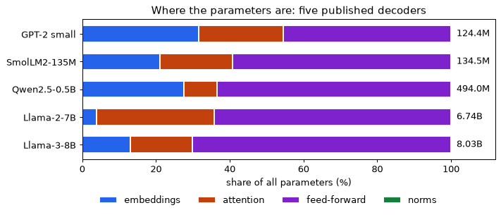
contexts = np.logspace(np.log10(512), np.log10(131072), 200)
matmul_g = np.full_like(contexts, matmul / GFLOP)
one_token_g = 4 * llama2.L * llama2.d * contexts / GFLOP
causal_avg_g = 2 * llama2.L * llama2.d * contexts / GFLOP

fig, ax = plt.subplots(figsize=(8, 5))
ax.plot(contexts, matmul_g, color="#1A2E4A", label="matrix multiplies, 2 N_matmul")
ax.plot(contexts, one_token_g, color="#C2410C",
        label="attention, one token at context t (4Ldt)")
ax.plot(contexts, matmul_g + one_token_g, color="#2563EB",
        label="total for that token")
ax.plot(contexts, causal_avg_g, color="#15803D", linestyle="--",
        label="attention, average over a causal sequence of length T (2LdT)")
# mark the crossovers; the labels sit on opposite sides so that they never overlap
for x, text, side in ((t_cross, f"t = {t_cross:,.0f}\n(6d = {6 * llama2.d:,})", "right"),
                      (T_cross, f"T = {T_cross:,.0f}\n(12d = {12 * llama2.d:,})", "left")):
    ax.axvline(x, color="#94A3B8", linewidth=1, linestyle=":")
    nudge = 0.95 if side == "right" else 1.05
    ax.text(x * nudge, 76, text, ha=side, fontsize=9, color="#475569")
ax.set_xscale("log")
ax.set_xlim(512, 131072)
ax.set_ylim(0, 85)
ax.set_xlabel("context length (tokens, log scale)")
ax.set_ylabel("forward GFLOP per token")
ax.set_title("Llama-2-7B: attention overtakes the matrix multiplies at about 6d")
ax.legend(loc="upper center", bbox_to_anchor=(0.5, -0.14), ncols=2, fontsize=9,
          frameon=False)
plt.tight_layout()
plt.show()
Read the plot from left to right. Up to a few thousand tokens the total hugs the flat line and the familiar “2 FLOPs per parameter per token” is accurate. The single-token attention line crosses the flat line at t = 25{,}205, and beyond it a long-context token costs more for attention than for all the weights of the model together; the causal average crosses twice as far out, at T = 50{,}410. Both curves are straight lines in t, so on this logarithmic axis they bend upwards: doubling the context doubles the attention term and leaves the matrix multiplies alone.
What you should see
- The counter agrees to the parameter with PyTorch for the module’s two decoders (3,801,344 and 727,424) and with the reference implementations for all five published models, and each count rounds to the size its authors quote: 124M, 135M, 0.49B, 6.7B and 8B.
- The non-embedding count is within 0.5% of the 12Ld^2 rule for GPT-2 small and Llama-2-7B, the two models built as the rule assumes (multi-head attention, a feed-forward network of about 8d^2), but 11% below it for SmolLM2-135M and 55% above it for Qwen2.5-0.5B: grouped-query attention removes up to 2d^2 per layer and a wide feed-forward network adds 3 d_{\text{ff}}/d - 8 units of d^2.
- Embeddings are a fifth to a third of the small models and under 4% of Llama-2-7B; Llama-3-8B’s larger, untied vocabulary brings it back to 13%.
- The KV cache follows the number of KV heads: 512 KiB per token for Llama-2-7B’s 32 heads, 128 KiB for Llama-3-8B’s 8; a single 4,096-token sequence at the Llama-2-7B shape costs 2 GiB, a sixth of the weights.
- Attention FLOPs are a rounding error at short context (2% at 512 tokens) and overtake the matrix multiplies beyond about 6d tokens of context for a single token (25,205 for Llama-2-7B) and beyond about 12d averaged over a causal sequence (50,410).
- Training costs 42.87 GFLOP per token for Llama-2-7B at T = 4{,}096 under the convention; the shortcut 6N_{\text{total}} gives 40.43, 5.7% low.
Try this
- Mixture of experts. Add two fields to
Cfg,n_expertsandtop_k, and change the counter so that each layer holdsn_expertscopies of the feed-forward network plus a router (a d \times n_{\text{experts}} matrix), whilen_matmulcounts onlytop_kexperts per layer, the ones a token actually passes through. Print total against active parameters for the Llama-2-7B shape with 8 experts and top-2 routing; you should find about 37.0B in total and 11.1B active (both embedding tables included). The concept is in Module 05, the engineering in Module 08. - A configuration you did not type. If you are online, fetch the configuration of
HuggingFaceTB/SmolLM2-360Mwithtransformers.AutoConfig.from_pretrained(a download of about 1 KB, no weights), build aCfgfrom its fields and confirm 361,821,120 parameters, then the same number fromLlamaForCausalLMon the meta device. - The cache against context length. Write a function that returns the KV-cache size of one sequence as a function of its length and plot it for the Llama-2-7B shape with 32, 8 and 1 KV heads, from 1,000 to 128,000 tokens, with a horizontal line at the 12.6 GiB of the weights. Read off the context length at which one sequence’s cache outweighs the model in each layout.
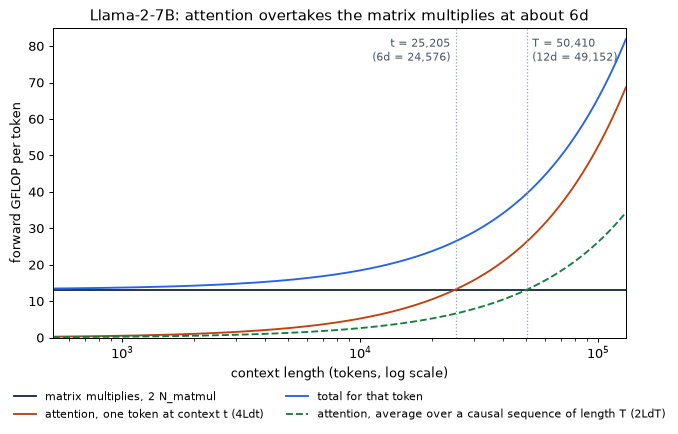
Lab 5 — Train a tiny GPT, sample from it, then remove the mask
Goal. Train a character-level decoder on generated maintenance records, compare its loss with source entropies, and test generated records. Then train the same architecture without a causal mask. Prefix-only scoring will reveal a failure that held-out window loss misses. The lab is self-contained and downloads no data.
Step 1: generate the records
QUICK = True trains for 300 causal steps and 200 unmasked steps. Set it to False
for FULL_STEPS = 1500 causal steps and the same 200 unmasked steps. Four CPU threads
keep the run comparable with the other labs; runtime depends on the machine. A full
run can take several minutes. The longer run gives copying more time to develop.
import collections
import json
import math
import random
import re
import time
import numpy as np
import matplotlib.pyplot as plt
import torch
import torch.nn as nn
import torch.nn.functional as F

QUICK = True
FULL_STEPS = 1500
torch.set_num_threads(4)
torch.manual_seed(0)
np.random.seed(0)
source_rng = random.Random(0)
specs = {
    "P": ("pump", "pressure", "bar", 0.5, 7.5, 2.0, 6.0),
    "T": ("tank", "level", "%", 2, 99, 10, 90),
    "C": ("compressor", "speed", "rpm", 2400, 3300, 2600, 3100),
    "H": ("exchanger", "outlet", "C", 35, 95, 40, 85),
    "V": ("valve", "position", "%", 0, 100, None, None),
}


def status_for(letter, value):
    low, high = specs[letter][-2:]
    if low is None:
        return "OK"
    return "LOW" if value < low else "HIGH" if value > high else "OK"


lines = []
for _ in range(12000):
    letter = source_rng.choice("PTCHV")
    identifier = f"{letter}-{source_rng.randint(0, 999):03d}"
    kind, quantity, unit, low, high, _, _ = specs[letter]
    value = (source_rng.uniform(low, high) if letter == "P"
             else source_rng.randint(low, high))
    shown = f"{value:.1f}" if letter == "P" else str(value)
    # Status is determined by the displayed value so records can be checked exactly.
    status = status_for(letter, float(shown))
    lines.append(f"{identifier} {kind} {quantity} {shown} {unit} "
                 f"{status} end {identifier}\n")
corpus = "".join(lines)
alphabet = sorted(set(corpus))
encode = {character: index for index, character in enumerate(alphabet)}
tokens = torch.tensor([encode[c] for c in corpus], dtype=torch.long)
split = int(0.9 * len(tokens))
train_data, valid_data = tokens[:split], tokens[split:]
vocab = len(alphabet)
print(f"mode: {'QUICK' if QUICK else 'FULL'}")
print(f"characters {len(corpus):,}, lines {len(lines):,}, vocabulary {vocab}")
print("".join(lines[:3]), end="")
mode: QUICK
characters 486,841, lines 12,000, vocabulary 46
H-776 exchanger outlet 91 C HIGH end H-776
H-041 exchanger outlet 51 C OK end H-041
V-497 valve position 51 % OK end V-497
Each closing identifier repeats the opening one. The status is a deterministic function of the displayed value. Thus the generator introduces uncertainty only in the record type, identifier and value. A split by character position may cut one record; it does not expose validation targets to training windows because windows stay within each split.
Step 2: reference entropies
Unigram and bigram entropy below are plug-in estimates from training characters. The generator entropy is calculated from the actual distribution of record types, numbers and rounded pressure values. Rounding a uniform pressure gives half-width bins at the two endpoints, rather than making all 71 printed values equally likely.
def entropy(probabilities):
    p = np.asarray(probabilities, dtype=float)
    p = p[p > 0]
    return float(-(p * np.log(p)).sum())


training_text = corpus[:split]
counts = collections.Counter(training_text)
unigram = entropy(np.array(list(counts.values())) / len(training_text))
pairs = collections.Counter(zip(training_text[:-1], training_text[1:]))
previous = collections.Counter(training_text[:-1])
bigram = -sum(n / (len(training_text) - 1) * math.log(n / previous[a])
              for (a, b), n in pairs.items())
mean_length, value_entropy = 0., 0.
for letter, (kind, quantity, unit, low, high, _, _) in specs.items():
    if letter == "P":
        values = np.arange(5, 76) / 10
        probabilities = np.full(71, 1 / 70)
        probabilities[[0, -1]] /= 2
    else:
        values = np.arange(low, high + 1)
        probabilities = np.full(len(values), 1 / len(values))
    value_entropy += entropy(probabilities) / 5
    for value, probability in zip(values, probabilities):
        shown = f"{value:.1f}" if letter == "P" else str(int(value))
        record = (f"{letter}-000 {kind} {quantity} {shown} {unit} "
                  f"{status_for(letter, float(value))} end {letter}-000\n")
        mean_length += len(record) * probability / 5
line_entropy = math.log(5) + math.log(1000) + value_entropy
true_floor = line_entropy / mean_length
no_copy_floor = (line_entropy + math.log(1000)) / mean_length
print(f"uniform {math.log(vocab):.3f}, unigram {unigram:.3f}, bigram {bigram:.3f}")
print(f"generator: {line_entropy:.3f} nats/line, {mean_length:.3f} chars/line")
print(f"true entropy {true_floor:.3f}, no-copy reference {no_copy_floor:.3f} nats/char")
uniform 3.829, unigram 3.410, bigram 1.717
generator: 13.392 nats/line, 40.558 chars/line
true entropy 0.330, no-copy reference 0.501 nats/char
The no-copy reference assumes that the equipment letter is known from the record but
the repeated three digits are predicted afresh. It adds log(1000) per line. It is a
reference for a restricted predictor, rather than the entropy of the complete source.
Step 3: the complete decoder and initialisation check
The model code is repeated here so this lab does not need variables from Lab 4. RoPE uses adjacent pairs and both key and value heads are expanded in contiguous groups.
def rope(x, base=10000.0):
    """x: (B, h, T, dk). Rotate pairs of dims by position-dependent angles."""
    B, h, T, dk = x.shape
    theta = base ** (-torch.arange(0, dk, 2, device=x.device) / dk)   # (dk/2,)
    ang = torch.arange(T, device=x.device)[:, None] * theta[None, :]   # (T, dk/2)
    cos, sin = ang.cos()[None, None], ang.sin()[None, None]
    x1, x2 = x[..., 0::2], x[..., 1::2]
    return torch.stack([x1 * cos - x2 * sin, x1 * sin + x2 * cos], dim=-1).flatten(-2)


class Attention(nn.Module):
    def __init__(self, d, n_heads, n_kv_heads, causal=True):
        super().__init__()
        self.h, self.kv, self.dk = n_heads, n_kv_heads, d // n_heads
        self.causal = causal
        self.wq = nn.Linear(d, d, bias=False)
        self.wk = nn.Linear(d, n_kv_heads * self.dk, bias=False)
        self.wv = nn.Linear(d, n_kv_heads * self.dk, bias=False)
        self.wo = nn.Linear(d, d, bias=False)

    def forward(self, x):
        B, T, d = x.shape
        q = self.wq(x).view(B, T, self.h, self.dk).transpose(1, 2)    # (B, h, T, dk)
        k = self.wk(x).view(B, T, self.kv, self.dk).transpose(1, 2)
        v = self.wv(x).view(B, T, self.kv, self.dk).transpose(1, 2)
        q, k = rope(q), rope(k)
        k = k.repeat_interleave(self.h // self.kv, dim=1)    # grouped-query: share KV
        v = v.repeat_interleave(self.h // self.kv, dim=1)
        y = F.scaled_dot_product_attention(q, k, v, is_causal=self.causal)
        return self.wo(y.transpose(1, 2).reshape(B, T, d))


class Block(nn.Module):
    def __init__(self, d, n_heads, n_kv_heads, d_ff, causal=True):
        super().__init__()
        self.n1, self.n2 = nn.RMSNorm(d), nn.RMSNorm(d)
        self.attn = Attention(d, n_heads, n_kv_heads, causal)
        self.w1 = nn.Linear(d, d_ff, bias=False)
        self.w3 = nn.Linear(d, d_ff, bias=False)
        self.w2 = nn.Linear(d_ff, d, bias=False)

    def forward(self, x):
        x = x + self.attn(self.n1(x))                           # pre-norm residual
        h = self.n2(x)
        return x + self.w2(F.silu(self.w1(h)) * self.w3(h))    # SwiGLU feed-forward


class Decoder(nn.Module):
    def __init__(self, vocab, d=256, layers=4, n_heads=8, n_kv_heads=2, d_ff=None,
                 causal=True):
        super().__init__()
        d_ff = d_ff or int(8 * d / 3)
        self.emb = nn.Embedding(vocab, d)
        self.blocks = nn.ModuleList(Block(d, n_heads, n_kv_heads, d_ff, causal)
                                    for _ in range(layers))
        self.norm = nn.RMSNorm(d)
        self.head = nn.Linear(d, vocab, bias=False)
        self.head.weight = self.emb.weight                          # tied embeddings
        nn.init.normal_(self.emb.weight, std=0.02)    # keeps step-0 logits small

    def forward(self, tokens):                                  # tokens: (B, T) ints
        x = self.emb(tokens)
        for b in self.blocks:
            x = b(x)
        return self.head(self.norm(x))                          # logits: (B, T, vocab)


def make_model(causal):
    torch.manual_seed(0)
    return Decoder(vocab=vocab, d=128, layers=4, n_heads=4, n_kv_heads=2,
                   causal=causal)


def batch(data, generator, B=32, T=128):
    starts = torch.randint(len(data) - T, (B,), generator=generator)
    windows = data[starts[:, None] + torch.arange(T + 1)]
    return windows[:, :-1], windows[:, 1:]


x0, y0 = batch(train_data, torch.Generator().manual_seed(1))
bad = make_model(True)
with torch.no_grad():
    nn.init.normal_(bad.emb.weight, std=1.0)
    bad_loss = F.cross_entropy(bad(x0).reshape(-1, vocab), y0.reshape(-1)).item()
good = make_model(True)
with torch.no_grad():
    good_loss = F.cross_entropy(good(x0).reshape(-1, vocab), y0.reshape(-1)).item()
print(f"parameters: {sum(p.numel() for p in good.parameters()):,}")
print(f"unit-scale tied embeddings: {bad_loss:.3f}")
print(f"std 0.02 embeddings: {good_loss:.3f}; uniform baseline {math.log(vocab):.3f}")
assert sum(p.numel() for p in good.parameters()) == 727424
del bad, good
parameters: 727,424
unit-scale tied embeddings: 115.321
std 0.02 embeddings: 3.881; uniform baseline 3.829
The unit-scale counterexample deliberately reinitialises the shared table; its exact
number depends on the draw. It demonstrates why an initial loss far above log(vocab)
deserves investigation before a training run.
Step 4: causal training
Validation uses ten fixed held-out batches each time, while training has its own random generator. The model has no dropout. Losses therefore compare the same validation windows across checkpoints. Elapsed time is omitted from the printed output so machine load does not obscure the numerical comparison.
@torch.no_grad()
def validation_loss(model):
    model.eval()
    generator = torch.Generator().manual_seed(2)
    losses = []
    for _ in range(10):
        x, y = batch(valid_data, generator)
        losses.append(F.cross_entropy(model(x).reshape(-1, vocab), y.reshape(-1)).item())
    return float(np.mean(losses))


def train(causal, steps):
    model = make_model(causal)
    optimiser = torch.optim.AdamW(model.parameters(), lr=3e-3,
                                 betas=(0.9, 0.95), weight_decay=0.1)
    generator = torch.Generator().manual_seed(1)
    curve = []
    for step in range(1, steps + 1):
        progress = max(0, (step - 50) / (steps - 50))
        scale = step / 50 if step <= 50 else 0.5 * (1 + math.cos(math.pi * progress))
        for group in optimiser.param_groups:
            group["lr"] = 3e-3 * scale
        model.train()
        x, y = batch(train_data, generator)
        loss = F.cross_entropy(model(x).reshape(-1, vocab), y.reshape(-1))
        optimiser.zero_grad(set_to_none=True)
        loss.backward()
        torch.nn.utils.clip_grad_norm_(model.parameters(), 1.0)
        optimiser.step()
        if step == 1 or step % 100 == 0 or step == steps:
            held_out = validation_loss(model)
            curve.append((step, loss.item(), held_out))
            print(f"step {step:4d}: train {loss.item():.3f}, validation {held_out:.3f}",
                  flush=True)
    return model, curve


causal, causal_curve = train(True, 300 if QUICK else FULL_STEPS)
step    1: train 3.881, validation 3.858
step  100: train 0.562, validation 0.567
step  200: train 0.540, validation 0.542
step  300: train 0.533, validation 0.532
QUICK need not learn the long-range copying rule. The longer schedule lets the loss
move below the no-copy reference, if the model learns to reuse the opening identifier.
Transition timing varies with floating-point arithmetic and schedule. If a full run
ends during the transition, try FULL_STEPS = 2000 and report the extra compute.
Step 5: sample and parse
Sample 32 independent sequences with a fixed sampling generator at temperature 0.8. Exclude the incomplete last line of each sample. Report malformed lines separately; identifier and status accuracy are conditional on the lines that satisfy the format.
@torch.no_grad()
def sample(model, count=32, steps=240):
    model.eval()
    generator = torch.Generator().manual_seed(3)
    sequence = torch.full((count, 1), encode["\n"], dtype=torch.long)
    for _ in range(steps):
        probabilities = (model(sequence[:, -128:])[:, -1] / 0.8).softmax(-1)
        next_token = torch.multinomial(probabilities, 1, generator=generator)
        sequence = torch.cat((sequence, next_token), dim=1)
    return ["".join(alphabet[i] for i in row) for row in sequence.tolist()]


pattern = re.compile(
    r"^([PTCHV])-(\d{3}) (\w+) (\w+) (\d+(?:\.\d)?) (\S+) "
    r"(OK|LOW|HIGH) end ([PTCHV]-\d{3})$")


def score_samples(texts):
    complete = [line for text in texts for line in text.split("\n")[1:-1]]
    parsed, copied, correct_status = 0, 0, 0
    for line in complete:
        match = pattern.fullmatch(line)
        if match is None:
            continue
        letter, digits, kind, quantity, shown, unit, status, closing = match.groups()
        spec = specs[letter]
        if (kind, quantity, unit) != spec[:3]:
            continue
        parsed += 1
        copied += closing == f"{letter}-{digits}"
        correct_status += status == status_for(letter, float(shown))
    print(f"complete {len(complete)}, well-formed {parsed} "
          f"({parsed / max(1, len(complete)):.1%})")
    print(f"among well-formed: identifier copied {copied / max(1, parsed):.1%}, "
          f"correct status {correct_status / max(1, parsed):.1%}")
    return dict(complete=len(complete), parsed=parsed, copied=copied,
                correct_status=correct_status)


causal_samples = sample(causal)
print(causal_samples[0])
causal_scores = score_samples(causal_samples)
P-201 pump pressure 4.6 bar OK end P-828
C-143 compressor speed 3096 rpm HIGH end C-583
T-238 tank level 40 % OK end T-413
P-172 pump pressure 4.7 bar OK end P-495
T-280 tank level 79 % OK end T-998
C-987 compressor speed 3325 rpm HIGH end
complete 176, well-formed 170 (96.6%)
among well-formed: identifier copied 0.0%, correct status 90.0%
Format, copying and status are distinct success criteria. A plausible record can have the wrong closing identifier. This synthetic parser establishes correctness only for the rules written here, rather than for a real maintenance decision.
Step 6: train without the mask and evaluate prefixes
Use the same initialisation and training-batch seed. Changing the causal flag is the only architecture change. A random held-out window supplies each prefix-only prediction with between eight and 127 actual prefix characters, never its target.
unmasked, unmasked_curve = train(False, 200)
unmasked_samples = sample(unmasked)
print("unmasked sample:")
print(unmasked_samples[0])
unmasked_scores = score_samples(unmasked_samples)


@torch.no_grad()
def prefix_loss(model, predictions=200):
    model.eval()
    generator = torch.Generator().manual_seed(5)
    losses = []
    for _ in range(predictions):
        start = int(torch.randint(len(valid_data) - 129, (), generator=generator))
        length = int(torch.randint(8, 128, (), generator=generator))
        prefix = valid_data[start:start + length][None]
        target = valid_data[start + length][None]
        losses.append(F.cross_entropy(model(prefix)[:, -1], target).item())
    return float(np.mean(losses))


causal_prefix, unmasked_prefix = prefix_loss(causal), prefix_loss(unmasked)
print(f"prefix-only loss: causal {causal_prefix:.3f}, unmasked {unmasked_prefix:.3f}")
print(f"window validation: causal {validation_loss(causal):.3f}, "
      f"unmasked {validation_loss(unmasked):.3f}")
step    1: train 3.907, validation 3.860
step  100: train 0.336, validation 0.338
step  200: train 0.011, validation 0.014
unmasked sample:

-iitir rrrerl rr aar e er 88888888888888888888878888  an e H-888 H-888 excharer r 89 % OK end T-888
H-78 exchanger outlet 888 C LOW end H-888
H-888 exchGH-8888 lve bale C OK end H-888
T-888 tanr level 88 % OK end T-880
H-883 exchanger outle
complete 83, well-formed 0 (0.0%)
among well-formed: identifier copied 0.0%, correct status 0.0%
prefix-only loss: causal 0.521, unmasked 1.291
window validation: causal 0.532, unmasked 0.014
The unmasked model can read most targets during window evaluation. The final input position is an exception, since its next-character target lies beyond the window. Prefix-only evaluation removes the leakage at every tested position. No held-out split can compensate for using future input when predicting a target.
Step 7: compare the curves
fig, ax = plt.subplots(figsize=(8, 4.5))
for name, curve, style in (("causal", causal_curve, "-"),
                            ("unmasked", unmasked_curve, "--")):
    values = np.asarray(curve)
    ax.plot(values[:, 0], values[:, 2], style, label=f"{name}, validation")
for level, name in ((math.log(vocab), "uniform"), (unigram, "unigram"),
                    (bigram, "bigram"), (no_copy_floor, "no-copy reference"),
                    (true_floor, "generator entropy")):
    ax.axhline(level, linewidth=0.8, alpha=0.5, label=f"{name}: {level:.3f}")
ax.set_xscale("log")
ax.set_xlabel("training step")
ax.set_ylabel("loss (nats per character)")
ax.set_title(f"Maintenance records: {'QUICK' if QUICK else 'FULL'} run")
ax.legend(fontsize=8)
plt.tight_layout()
plt.show()
metrics = dict(mode="QUICK" if QUICK else "FULL", causal_curve=causal_curve,
               unmasked_curve=unmasked_curve, causal_scores=causal_scores,
               unmasked_scores=unmasked_scores, causal_prefix=causal_prefix,
               unmasked_prefix=unmasked_prefix, true_floor=true_floor,
               no_copy_floor=no_copy_floor)
with open("m06-lab5-metrics.json", "w", encoding="utf-8") as stream:
    json.dump(metrics, stream, indent=2)
What you should see
The causal loss crosses the unigram and bigram references while format and local regularities improve. Compare the measured copying share with whether loss crosses the no-copy reference. The unmasked model’s window loss can become much lower while its prefix-only loss and generated records expose the information leak. The printed outputs are from the executed QUICK run; FULL observations are reported separately in the text.
With QUICK = False, the executed 1500-step causal run reached validation loss 0.399
and prefix-only loss 0.394. It generated 172 complete lines: all parsed, 155 copied
the opening identifier correctly (90.1%), and 171 had the correct status (99.4%).
Its validation loss fell below the no-copy reference after about 1000 steps. The
unmasked control remained at window loss 0.014 and prefix-only loss 1.291, and none
of its 83 complete generated lines parsed. The QUICK output fences above are retained
so the default code and displayed outputs describe the same run.
Try this
- Use a public-domain text of 0.2–2 MB; recompute the vocabulary and empirical entropies.
- Reduce the context to 32 characters and inspect which parts of the opening identifier remain visible when each closing character is predicted. Do not assume one floor applies to every record length: this corpus contains different formats and lengths.
- Repeat sampling at temperatures 0.3 and 1.5 and score format, copying and status again.
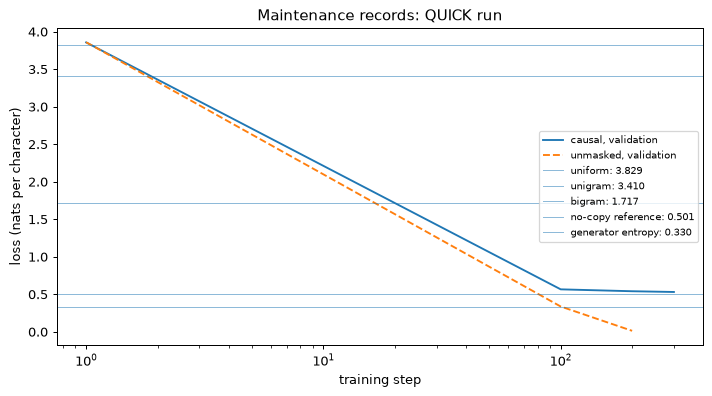
Lab 6 — Find an induction head
Goal. Train an attention-only transformer on repeated random segments, measure previous-token and induction attention, and intervene on the heads. Compare a two-layer model with a one-layer control. Everything is generated locally; no model is downloaded.
Step 1: generate a task whose copy distance varies
Draw a 64-token sequence and a segment length from 10 through 32. Repeat the first
segment immediately after itself. The first token of the repetition is not predictable
from its prefix; subsequent repeated tokens are. Targets are shifted one token ahead,
so a predictable target at position j is evaluated from query position j - 1.
import json
import numpy as np
import matplotlib.pyplot as plt
import torch
import torch.nn as nn
import torch.nn.functional as F

np.random.seed(0)
torch.manual_seed(0)
torch.set_num_threads(4)
VOCAB, LENGTH, STEPS = 64, 64, 1500


def repeated_batch(generator, count=64):
    tokens = torch.randint(VOCAB, (count, LENGTH), generator=generator)
    segment = torch.randint(10, 33, (count,), generator=generator)
    predictable = torch.zeros_like(tokens, dtype=torch.bool)
    for row, n in enumerate(segment.tolist()):
        tokens[row, n:2 * n] = tokens[row, :n].clone()
        predictable[row, n + 1:2 * n] = True
    return tokens[:, :-1], tokens[:, 1:], predictable[:, 1:], segment


x, y, predictable, segment = repeated_batch(torch.Generator().manual_seed(1))
print("inputs", tuple(x.shape), "targets", tuple(y.shape))
print("segment lengths:", segment[:8].tolist())
print(f"predictable target share: {predictable.float().mean():.3f}")
assert all(torch.equal(x[row, n:2 * n - 1], x[row, :n - 1])
           for row, n in enumerate(segment.tolist()))
inputs (64, 63) targets (64, 63)
segment lengths: [13, 13, 21, 25, 16, 22, 13, 14]
predictable target share: 0.295
A fixed copy distance could be solved by a position-based rule. Varying the distance makes the model find a matching earlier token and use the token that followed it. Random token collisions can still make the next token ambiguous; this is a task distribution, rather than a guarantee that every repeated token has a unique match.
Step 2: attention with accessible weights and head outputs
Explicit softmax lets the lab inspect attention and zero head outputs before the output projection. Ablation removes the whole head’s contribution, not just one entry of its attention map. The model has no feed-forward sublayers.
def rotary(x):
    T, dk = x.shape[-2:]
    frequencies = 10000.0 ** (-torch.arange(0, dk, 2) / dk)
    angles = torch.arange(T)[:, None] * frequencies[None]
    cosine, sine = angles.cos()[None, None], angles.sin()[None, None]
    first, second = x[..., 0::2], x[..., 1::2]
    return torch.stack((first * cosine - second * sine,
                        first * sine + second * cosine), dim=-1).flatten(-2)


class InspectableBlock(nn.Module):
    def __init__(self, width=64, heads=4):
        super().__init__()
        self.heads, self.dk = heads, width // heads
        self.norm = nn.RMSNorm(width)
        self.qkv = nn.Linear(width, 3 * width, bias=False)
        self.output = nn.Linear(width, width, bias=False)

    def forward(self, x, zero_heads=()):
        B, T, d = x.shape
        q, k, v = (a.reshape(B, T, self.heads, self.dk).transpose(1, 2)
                   for a in self.qkv(self.norm(x)).chunk(3, dim=-1))
        q, k = rotary(q), rotary(k)
        scores = q @ k.transpose(-1, -2) / self.dk ** 0.5
        future = torch.ones(T, T, dtype=torch.bool).triu(1)
        weights = scores.masked_fill(future, -torch.inf).softmax(-1)
        head_output = weights @ v
        if zero_heads:
            head_output = head_output.clone()
            head_output[:, list(zero_heads)] = 0
        merged = head_output.transpose(1, 2).reshape(B, T, d)
        return x + self.output(merged), weights


class CopyModel(nn.Module):
    def __init__(self, layers):
        super().__init__()
        self.embedding = nn.Embedding(VOCAB, 64)
        nn.init.normal_(self.embedding.weight, std=0.02)
        self.blocks = nn.ModuleList(InspectableBlock() for _ in range(layers))
        self.norm = nn.RMSNorm(64)
        self.head = nn.Linear(64, VOCAB, bias=False)

    def forward(self, tokens, ablate=None):
        x, maps = self.embedding(tokens), []
        for layer, block in enumerate(self.blocks):
            x, weights = block(x, (ablate or {}).get(layer, ()))
            maps.append(weights)
        return self.head(self.norm(x)), maps


model = CopyModel(2)
print(f"two-layer parameters: {sum(p.numel() for p in model.parameters()):,}")
two-layer parameters: 41,152
Step 3: train and separate predictable targets
Train on every target, not just the repeated region. Report predictable and unpredictable losses on fixed fresh batches. The latter provide a useful control: random non-copy targets should remain difficult even after copying improves.
@torch.no_grad()
def evaluate(model, count=256, seed=9, ablate=None):
    model.eval()
    x, y, predictable, segment = repeated_batch(
        torch.Generator().manual_seed(seed), count)
    logits, maps = model(x, ablate)
    losses = F.cross_entropy(logits.reshape(-1, VOCAB), y.reshape(-1),
                             reduction="none").reshape_as(y)
    return (losses[predictable].mean().item(),
            losses[~predictable].mean().item(), maps, predictable, segment, x)


def fit(layers):
    torch.manual_seed(0)
    model = CopyModel(layers)
    optimiser = torch.optim.AdamW(model.parameters(), lr=1e-3, weight_decay=0)
    generator = torch.Generator().manual_seed(1)
    curve = []
    for step in range(1, STEPS + 1):
        model.train()
        x, y, _, _ = repeated_batch(generator)
        logits, _ = model(x)
        loss = F.cross_entropy(logits.reshape(-1, VOCAB), y.reshape(-1))
        optimiser.zero_grad(set_to_none=True)
        loss.backward()
        optimiser.step()
        if step == 1 or step % 100 == 0:
            repeated, random_loss, *_ = evaluate(model, count=64)
            curve.append((step, repeated, random_loss))
            print(f"layers {layers}, step {step:4d}: copy {repeated:.3f}, "
                  f"other {random_loss:.3f}", flush=True)
    return model, curve


two_layer, two_curve = fit(2)
layers 2, step    1: copy 4.290, other 4.307
layers 2, step  100: copy 3.917, other 4.211
layers 2, step  200: copy 3.771, other 4.221
layers 2, step  300: copy 3.639, other 4.231
layers 2, step  400: copy 3.524, other 4.256
layers 2, step  500: copy 3.401, other 4.281
layers 2, step  600: copy 2.871, other 4.346
layers 2, step  700: copy 1.197, other 4.513
layers 2, step  800: copy 0.829, other 4.424
layers 2, step  900: copy 0.579, other 4.361
layers 2, step 1000: copy 0.436, other 4.332
layers 2, step 1100: copy 0.374, other 4.324
layers 2, step 1200: copy 0.346, other 4.305
layers 2, step 1300: copy 0.374, other 4.285
layers 2, step 1400: copy 0.338, other 4.287
layers 2, step 1500: copy 0.304, other 4.288
Step 4: quantify where heads attend
The previous-token score averages weight from query t to key t - 1 over all
non-initial queries. For a predictable query t, the earlier successor is key
t - n + 1, with n the segment length. The induction score averages weight on
that key. Compute scores over 256 fresh sequences, rather than selecting a flattering
single example.
@torch.no_grad()
def head_scores(model):
    repeated, random_loss, maps, predictable, segment, x = evaluate(model)
    previous_scores, induction_scores = [], []
    batch_ids, query_ids = predictable.nonzero(as_tuple=True)
    key_ids = query_ids - segment[batch_ids] + 1
    for layer, weights in enumerate(maps):
        previous = weights.diagonal(offset=-1, dim1=-2, dim2=-1).mean(dim=(0, 2))
        induction = weights[batch_ids, :, query_ids, key_ids].mean(dim=0)
        previous_scores.append(previous.numpy())
        induction_scores.append(induction.numpy())
        print(f"layer {layer}: previous "
              + " ".join(f"{v:.3f}" for v in previous.tolist()))
        print(f"layer {layer}: induction "
              + " ".join(f"{v:.3f}" for v in induction.tolist()))
    print(f"held-out copy loss {repeated:.3f}, other loss {random_loss:.3f}")
    return previous_scores, induction_scores, maps, segment


previous, induction, maps, segments = head_scores(two_layer)
previous_head = int(np.argmax(previous[0]))
induction_head = int(np.argmax(induction[1]))
fig, axes = plt.subplots(1, 2, figsize=(10, 4))
for ax, layer, head, title in (
        (axes[0], 0, previous_head, "strongest layer-0 previous-token score"),
        (axes[1], 1, induction_head, "strongest layer-1 induction score")):
    pattern = maps[layer][0, head].numpy()
    image = ax.imshow(pattern, vmin=0, vmax=1, origin="upper", cmap="Blues")
    ax.set_xlabel("key position")
    ax.set_ylabel("query position")
    ax.set_title(f"{title}\nhead {head}, segment length {int(segments[0])}", fontsize=9)
    fig.colorbar(image, ax=ax, fraction=0.046)
plt.tight_layout()
plt.show()
layer 0: previous 0.631 0.300 0.119 0.110
layer 0: induction 0.000 0.000 0.001 0.001
layer 1: previous 0.052 0.035 0.041 0.037
layer 1: induction 0.927 0.920 0.935 0.922
held-out copy loss 0.286, other loss 4.297
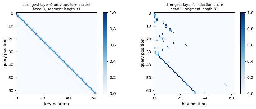
Step 5: intervene on every head
Evaluate each intervention on the same 512 fresh sequences. A larger loss means the head’s contribution mattered to this trained model on this distribution. It does not prove that the head is the unique implementation of a human-defined concept.
baseline = evaluate(two_layer, count=512, seed=11)[0]
print(f"baseline copy loss {baseline:.3f}")
ablations = []
for layer in range(2):
    for head in range(4):
        loss = evaluate(two_layer, count=512, seed=11, ablate={layer: [head]})[0]
        ablations.append((layer, head, loss))
        print(f"zero layer {layer}, head {head}: {loss:.3f}, change {loss - baseline:+.3f}")
    loss = evaluate(two_layer, count=512, seed=11, ablate={layer: list(range(4))})[0]
    print(f"zero all heads in layer {layer}: {loss:.3f}")
baseline copy loss 0.270
zero layer 0, head 0: 2.866, change +2.596
zero layer 0, head 1: 1.373, change +1.103
zero layer 0, head 2: 2.855, change +2.585
zero layer 0, head 3: 2.811, change +2.541
zero all heads in layer 0: 4.518
zero layer 1, head 0: 2.265, change +1.995
zero layer 1, head 1: 1.986, change +1.716
zero layer 1, head 2: 2.513, change +2.242
zero layer 1, head 3: 1.873, change +1.603
zero all heads in layer 1: 4.399
Removing a whole layer is an intervention outside the trained state distribution. Compare it with single-head interventions and the attention scores instead of treating any one loss change as a complete explanation.
Step 6: a one-layer control
Use the same batch generator, training steps and optimiser. A one-layer model has fewer parameters and only one attention stage, so the comparison changes both capacity and available computation. It tests this particular setup, not a universal impossibility theorem about one-layer transformers.
one_layer, one_curve = fit(1)
one_previous, one_induction, _, _ = head_scores(one_layer)
fig, ax = plt.subplots(figsize=(8, 4))
for name, curve in (("two layers", two_curve), ("one layer", one_curve)):
    curve = np.asarray(curve)
    ax.plot(curve[:, 0], curve[:, 1], label=f"{name}, predictable")
ax.axhline(math_log_vocab := float(np.log(VOCAB)), color="grey", linestyle=":",
           label=f"uniform guess: {math_log_vocab:.2f}")
ax.set_xlabel("training step")
ax.set_ylabel("held-out loss (nats per token)")
ax.set_title("Copying a variable-distance repeated segment")
ax.legend()
plt.tight_layout()
plt.show()
metrics = dict(two_curve=two_curve, one_curve=one_curve,
               previous=[a.tolist() for a in previous],
               induction=[a.tolist() for a in induction],
               ablations=ablations, baseline=baseline,
               one_induction=[a.tolist() for a in one_induction])
with open("m06-lab6-metrics.json", "w", encoding="utf-8") as stream:
    json.dump(metrics, stream, indent=2)
layers 1, step    1: copy 4.259, other 4.303
layers 1, step  100: copy 4.068, other 4.172
layers 1, step  200: copy 3.681, other 4.218
layers 1, step  300: copy 3.547, other 4.223
layers 1, step  400: copy 3.474, other 4.234
layers 1, step  500: copy 3.436, other 4.232
layers 1, step  600: copy 3.433, other 4.224
layers 1, step  700: copy 3.378, other 4.242
layers 1, step  800: copy 3.378, other 4.237
layers 1, step  900: copy 3.353, other 4.244
layers 1, step 1000: copy 3.339, other 4.240
layers 1, step 1100: copy 3.331, other 4.248
layers 1, step 1200: copy 3.337, other 4.242
layers 1, step 1300: copy 3.334, other 4.243
layers 1, step 1400: copy 3.324, other 4.240
layers 1, step 1500: copy 3.317, other 4.240
layer 0: previous 0.025 0.031 0.024 0.032
layer 0: induction 0.068 0.065 0.068 0.063
held-out copy loss 3.338, other loss 4.243
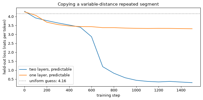
What you should see
Compare the copying-loss curves, attention scores and ablation effects. In this task the two-layer architecture can compose earlier-token information with a later lookup. The one-layer control tests how much that composition helps. Heads with modest attention scores can still affect outputs through their value and output projections; a heat map alone is incomplete evidence. The printed numbers above come from this lab’s execution, and may differ in the last digits or transition timing on another machine.
Try this
- Fix the segment length at 32 and compare the one-layer control with variable distance.
- Add SwiGLU sublayers and compare loss curves at both equal width and similar parameter count. Report which comparison is being made.
- Repeat training with seeds 1 and 2. Check whether copying appears and which heads carry the measured patterns; head numbers need not have stable roles across seeds.
Exercises
Use natural logarithms and count one multiply-add as two FLOPs. The calculations use the conventions of Section 11. Attempt each exercise before opening its solution.
Explain why the first causal attention output is exactly the first value vector for any finite query and key. What information can its next-token prediction use?
Show solution
Only the first key is visible. Softmax over its single score is e^s/e^s=1, so the output is \mathbf{v}_1. Every later layer at that position has the same information boundary. Its prediction can depend on the first token and positional information, but cannot use any later token. This does not force a particular loss: an initial token could make its successor highly predictable in some sources.
Extend the three-token example with \mathbf{q}_4=\mathbf{k}_4=(1,-1). Remove the causal mask and use the four-by-four identity as the value matrix. Calculate each output row to three decimals. Explain the effect on the first three rows and the weight of an orthogonal key. Which rows would remain unchanged if the mask were restored?
Show solution
The unscaled score rows are (1,0,1,1), (0,1,1,-1), (1,1,2,0) and (1,-1,0,2). Divide each by \sqrt2. The four possible exponentials are 1, e^{1/\sqrt2}=2.028115, e^{-1/\sqrt2}=0.493069 and e^{\sqrt2}=4.113250. Normalising each row gives
Because \mathbf{V}=\mathbf{I}, \mathbf{O}=\mathbf{P}. The fourth key adds a positive exponential to every unmasked denominator, changing every earlier row. It is orthogonal to query three yet receives weight 0.109: a zero score has exponential one, rather than zero. With the causal mask, rows one through three cannot see key four and retain their previous weights, padded by a zero fourth component.
Describe what unscaled dot products of independent unit-variance queries and keys do at head width 128. Explain the consequence for learning query and key projections.
Show solution
Their variance is 128 and standard deviation \sqrt{128}=11.31. Such large random score gaps can make softmax nearly one-hot. Its Jacobian entries p_i(1-p_i) and -p_i p_j then become small, reducing the score gradients that reach query and key projections. Dividing scores by \sqrt{128} restores unit variance under the stated independence assumptions. It does not force trained scores to remain unit-variance.
Let \mathbf{P} be a permutation matrix. Prove that unmasked self-attention without positions obeys \operatorname{Attention}(\mathbf{P}\mathbf{X})= \mathbf{P}\operatorname{Attention}(\mathbf{X}). Also prove that jointly permuting keys and values leaves outputs fixed when queries are fixed. Does a fixed causal mask preserve the first identity for arbitrary permutations?
Show solution
Linear projection gives \mathbf{Q}'=\mathbf{P}\mathbf{Q}, \mathbf{K}'=\mathbf{P}\mathbf{K} and \mathbf{V}'=\mathbf{P}\mathbf{V}. Thus the scores become \mathbf{S}'=\mathbf{P}\mathbf{S}\mathbf{P}^{\top}. Permuting rows reorders independent softmax computations. Permuting columns reorders each row’s exponentials without changing its denominator. Consequently, \softmax(\mathbf{S}')=\mathbf{P}\softmax(\mathbf{S})\mathbf{P}^{\top} and
With fixed queries and jointly permuted keys/values, the scores are \mathbf{S}\mathbf{P}^{\top}. Their softmax is \softmax(\mathbf{S})\mathbf{P}^{\top}, and multiplication by \mathbf{P}\mathbf{V} cancels the permutation. A fixed causal mask is different: it is tied to sequence indices and generally does not equal its permuted version. Therefore arbitrary permutations do not preserve the masked identity. Unmasked attention without position information is equivariant to token order; position encodings or an order-dependent mask supply information that the content set lacks.
Write the pre-norm and post-norm residual updates. Identify the direct identity path and describe what it does, and does not, imply about gradients through many layers.
Show solution
Pre-norm is \mathbf{x}_{\ell+1}=\mathbf{x}_{\ell}+ F_{\ell}(\operatorname{Norm}(\mathbf{x}_{\ell})). Post-norm is \mathbf{x}_{\ell+1}=\operatorname{Norm}(\mathbf{x}_{\ell}+F_{\ell}(\mathbf{x}_{\ell})). The pre-norm Jacobian is an identity plus the sublayer derivative. A direct residual route crosses no intermediate normalisation Jacobians. In post-norm those Jacobians also act on the residual route. Pre-norm therefore supplies a simpler gradient path, but does not guarantee that all gradients are bounded or nonzero: branches can be poorly scaled or cancel. A final output norm also has its own derivative.
Write RoPE as a block-diagonal matrix of two-dimensional rotations. Prove the relative-position dot-product identity and norm preservation. Explain what happens to the output if values are also rotated at their absolute positions.
Show solution
For pair frequency \theta_i, use
Multiplying two blocks and using the angle-addition formulas gives \mathbf{R}(a)\mathbf{R}(b)=\mathbf{R}(a+b). Transposition gives \mathbf{R}(a)^{\top}=\mathbf{R}(-a). Hence block by block, \mathbf{R}_t^{\top}\mathbf{R}_s=\mathbf{R}_{s-t} and (\mathbf{R}_t\mathbf{q})^{\top}(\mathbf{R}_s\mathbf{k}) =\mathbf{q}^{\top}\mathbf{R}_{s-t}\mathbf{k}. Also \mathbf{R}_t^{\top}\mathbf{R}_t=\mathbf{I}, so \|\mathbf{R}_t\mathbf{q}\|^2=\mathbf{q}^{\top}\mathbf{q}. Rotated values would give \mathbf{o}_t=\sum_s p_{ts}\mathbf{R}_s\mathbf{v}_s. A common shift by c leaves the weights unchanged but transforms the output into \mathbf{R}_c\mathbf{o}_t. The score remains relative, while the output coordinates carry an absolute rotation. Ordinary RoPE leaves values unrotated.
A model has learned absolute positions for only 1024 positions and receives 2000 tokens. Contrast its failure with a RoPE model trained at length 1024.
Show solution
An embedding table of exactly 1024 rows cannot index later positions. A larger table with untrained later rows avoids the index error but does not give learned positional representations there. RoPE defines rotations beyond the training length, so it can execute. However, longer relative offsets expose untrained angular combinations and more competing keys. Mathematical definition beyond 1024 does not establish reliable long-context performance; extension requires suitable training and evaluation.
Give two reasons a bidirectional masked-language model is not immediately a left-to-right next-token generator.
Show solution
Its objective predicts selected missing tokens using context on both sides, rather than every successor from a prefix. Generation lacks that right-hand context. Its ordinary unmasked-position logits also were not trained as next-token distributions. One can build iterative masked-token generation or adapt the objective, but neither is the unchanged causal next-token procedure used here.
Compare 32-query-head, eight-KV-head GQA with full multi-head attention at the same width and depth. State which projections and stored inference tensors shrink by four, and which leading compute terms remain unchanged.
Show solution
Key and value projection output widths shrink from d to d/4, so each has a quarter of its previous weights. Retained keys and values also shrink fourfold. Query/output projections and the FFN remain unchanged. Every query head still scores every visible key and mixes a value vector, so leading query-key and probability-value FLOPs remain unchanged. Overall compute still falls somewhat because key/value projection work is smaller.
Explain why replacing dense attention with FlashAttention preserves a trained model’s function, while adding a sliding window generally changes it.
Show solution
FlashAttention computes the same visible scores, softmax and weighted sum in tiles; only floating-point ordering and execution details differ. A sliding window removes visible keys and changes both the softmax denominator and weighted sum. A full-attention checkpoint therefore needs adaptation and evaluation for the proposed window, rather than treating the change as an equivalent kernel substitution.
Process scores (2,1,3,0) and scalar values (1,2,3,4) in two blocks of two. Calculate the running maximum, normaliser and accumulator after each block. Check the output against a direct softmax-weighted average.
Show solution
After block one, m=2, \ell=1+e^{-1}=1.367879 and a=1+2e^{-1}=1.735759. Block two raises the maximum to 3, requiring old contributions to be multiplied by e^{-1}. Then
Their ratio is approximately 2.471. Direct exponentials on the maximum-three scale are (e^{-1},e^{-2},1,e^{-3}). Their sum is the same \ell' and their value-weighted sum is e^{-1}+2e^{-2}+3+4e^{-3}=a'. This checks the result without rounding weights before multiplication.
Count a tied decoder with vocabulary 4096, width 256, four layers, eight query heads, two KV heads, FFN width \lfloor8(256)/3\rfloor and bias-free RMSNorm. Itemise each component and explain its departure from 12Ld^2.
Show solution
The head width is 32 and KV projection width 64. The tied vocabulary table has 4096(256)=1{,}048{,}576 parameters. Per layer, query/output matrices contain 2(256^2)=131{,}072 and key/value matrices 2(256)(64)=32{,}768, giving attention 163,840. FFN width is 682, so its three matrices contain 3(256)(682)=523{,}776. Two norms add 512. One layer has 688,128; four have 2,752,512. Add 256 final-norm gains and the vocabulary table to obtain 3,801,344.
The rule 12Ld^2=3{,}145{,}728 excludes embeddings and assumes full multi-head attention. GQA saves 98,304 per layer. Rounding FFN width saves another 512 per layer, while two norms add 512 back. Thus blocks total 3{,}145{,}728-4(98{,}304) =2{,}752{,}512. Embeddings and final norm account for the remaining difference.
Use the Llama-2-7B-shaped counts from Section 11, two trillion training tokens, sequence length 4096 and a supplied budget of 184,320 GPU-hours. Compute model FLOPs with 6N_{\text{total}}D and with the series convention. Convert each to sustained FLOP/s per GPU and utilisation against a supplied 312 TFLOP/s peak. Explain what this utilisation estimate omits.
Show solution
Set N_{\text{total}}=6{,}738{,}415{,}616 and N_{\text{matmul}}=6{,}607{,}343{,}616. The quick count is 6N_{\text{total}}D=8.08610\times10^{22} FLOPs. The weight term is 7.92881\times10^{22} and the causal attention term 6(32)(4096)(4096)(2\times10^{12})=6.44245\times10^{21}. Their sum is 8.57306\times10^{22} FLOPs.
The supplied GPU-hours equal 184{,}320(3600)=663{,}552{,}000 GPU-seconds. Dividing gives approximately 1.219\times10^{14} and 1.292\times10^{14} FLOP/s per GPU. Divide by 312\times10^{12} to get 39.1% and 41.4% model FLOP utilisation. The quick count charges lookup weights and omits attention; those errors partly cancel, leaving it 5.7% low here. Neither model count includes checkpoint recomputation, optimiser operations, evaluation, downtime or communication. This is model FLOP utilisation, rather than a direct hardware activity measurement.
Training and validation losses fall to 0.02 nats per character unusually quickly. Name two leakage bugs and an intervention that tests the information boundary.
Show solution
A missing/reversed causal mask exposes successor tokens. Unshifted targets ask the model to reproduce its current input. Inspect input/target pairs, then change a future token while keeping the prefix fixed. In a causal next-token model, earlier logits must remain unchanged. Prefix-only evaluation and generation supply independent checks. Low held-out window loss alone does not distinguish either bug from successful learning.
Implement explicit causal attention and compare its outputs with PyTorch SDPA. For batch one, eight heads, head width 64 and float32, calculate score storage at lengths 512, 2048 and 4096 and time both implementations. Optionally compare GPU peak allocated memory at 512, 2048 and 8192, reporting the selected backend.
Show solution
The explicit implementation below is self-contained. Numerical comparison is performed before timing; timing excludes random input construction. A warmup avoids charging one implementation for first-call setup alone. Results remain machine-dependent.
import time
import torch
import torch.nn.functional as F

torch.manual_seed(0)
torch.set_num_threads(4)


def explicit(q, k, v):
    T = q.shape[-2]
    future = torch.ones(T, T, dtype=torch.bool, device=q.device).triu(1)
    scores = q @ k.transpose(-1, -2) / q.shape[-1] ** 0.5
    return scores.masked_fill(future, -torch.inf).softmax(-1) @ v


def fused(q, k, v):
    return F.scaled_dot_product_attention(q, k, v, is_causal=True)


with torch.no_grad():
    for T in (512, 2048, 4096):
        q, k, v = (torch.randn(1, 8, T, 64) for _ in range(3))
        reference, actual = explicit(q, k, v), fused(q, k, v)
        error = (reference - actual).abs().max().item()
        assert error < 1e-5
        print(f"T={T}: score storage {8 * T * T * 4 / 2**20:.0f} MiB, "
              f"max difference {error:.2e}")
        for name, function in (("explicit", explicit), ("SDPA", fused)):
            function(q, k, v)
            started = time.perf_counter()
            for _ in range(3):
                function(q, k, v)
            print(f"  {name}: {(time.perf_counter() - started) / 3:.4f} s")
The score tensors alone contain 8, 128 and 512 MiB. At 8192 positions they contain 2 GiB. The explicit implementation also holds softmax output and temporaries, so peak memory exceeds the score tensor’s size. SDPA’s memory depends on its selected implementation, rather than the function name alone.
For an optional GPU experiment, allocate inputs before resetting peak statistics. Measure incremental live allocation, synchronising around timing and memory queries. Large explicit runs may exceed available memory; an out-of-memory result is a capacity measurement, not a failed correctness test.
from torch.nn.attention import SDPBackend, sdpa_kernel

for T in (512, 2048, 8192):
    q, k, v = (torch.randn(1, 8, T, 64, device="cuda", dtype=torch.float16)
               for _ in range(3))
    for name, function in (("explicit", explicit), ("FlashAttention SDPA", fused)):
        torch.cuda.synchronize()
        baseline = torch.cuda.memory_allocated()
        torch.cuda.reset_peak_memory_stats()
        with torch.no_grad(), sdpa_kernel(SDPBackend.FLASH_ATTENTION):
            result = function(q, k, v)
        torch.cuda.synchronize()
        extra = torch.cuda.max_memory_allocated() - baseline
        print(T, name, "incremental peak MiB", extra / 2**20)
        del result
The explicit branch ignores the backend selection; the SDPA branch requires a supported FlashAttention backend. A backend error should be reported rather than silently replaced by a different implementation. Restore the fused call in the decoder after comparison.
Self-check quiz
Choose one answer for each question. Revisit the relevant concept section after a mistake.
Guided reading
Reading 1
Vaswani, A., Shazeer, N., Parmar, N., Uszkoreit, J., Jones, L., Gomez, A. N., Kaiser, Ł., Polosukhin, I. “Attention is all you need.” NeurIPS, 2017. Paper.
Why read it. The original; with this module behind you, every equation in its model section is familiar, and the differences from the modern block (post-norm, sinusoids, ReLU, encoder-decoder) become visible.
What to read. Read Section 3 (Model Architecture) in full and Section 4 (Why Self-Attention) with Table 1. Skim Section 5 (Training), stopping at the learning-rate formula with its warmup. Look only at Table 3’s ‘base’ and ‘big’ rows in Section 6; skip the remaining results and the conclusion.
Questions to answer while reading
- Find the footnote that justifies the 1/sqrt(d_k) scale. What assumption does it make, and is it the one used in Section 2 of this module?
- Table 1 compares complexity per layer. For which sequence lengths n (relative to d) is a self-attention layer cheaper than a recurrent one?
- Is the paper’s block pre-norm or post-norm? Quote the sublayer equation and connect it to the warmup in the learning-rate formula.
- Estimate the base model’s parameters with this module’s rules (d = 512, d_ff = 2,048, 6 encoder layers at 12d^2, 6 decoder layers at 16d^2, one shared embedding of about 37,000 x 512) and compare with the 65M of Table 3. (About 63M.)
- Which of the three shapes of Section 7 is this model, and where do its cross-attention keys and values come from?
Reading 2
Su, J., Lu, Y., Pan, S., Murtadha, A., Wen, B., Liu, Y. “RoFormer: Enhanced transformer with rotary position embedding.” arXiv:2104.09864, 2021. Paper.
Why read it. The derivation of RoPE by its authors, in the complex form Section 6 used, with the long-term decay property that Lab 2 plotted.
What to read. Read the formulation of the goal (a score that depends only on the relative position), the 2D derivation with complex numbers, the general form with the block-diagonal rotation matrix, and the efficient element-wise implementation and the long-term decay property. Skip the combination with linear attention and the experiments.
Questions to answer while reading
- The paper asks for functions f_q, f_k with <f_q(x_m, m), f_k(x_n, n)> = g(x_m, x_n, m - n). Write this in this module’s notation (q, k, t, s).
- Compare the paper’s element-wise implementation with the module’s rope() function. Which dimensions does each pair together, and why does the convention matter when weights are moved between implementations?
- State the long-term decay property in your own words and compare it with Lab 2’s curve for q = k = all ones.
Reading 3
Dao, T., Fu, D. Y., Ermon, S., Rudra, A., Ré, C. “FlashAttention: Fast and memory-efficient exact attention with IO-awareness.” NeurIPS, 2022. Paper.
Why read it. The paper that made attention’s memory linear in sequence length without approximation; its Algorithm 1 is Lab 3, and its background section is the clearest short account of why attention is memory-bound.
What to read. Read Section 2 (the GPU memory hierarchy, the standard implementation as Algorithm 0) and Section 3.1 (tiling, recomputation, Algorithm 1), and the statement of the IO-complexity theorem in Section 3.2 without its proof. Skim the block-sparse extension and look at one speed-up figure in the experiments.
Questions to answer while reading
- Map Algorithm 1’s updates of m and l onto the online-softmax recurrences of Section 10. Which line performs the rescaling by exp(m - m’)?
- The paper gives Theta(N d + N^2) HBM accesses for standard attention and Theta(N^2 d^2 / M) for FlashAttention, with M the SRAM size. Show that the ratio is about M / d^2 when N >> d, and evaluate it for d = 64 and M = 100 KB of fp16 values (about 51,200 elements): about 12.
- Why does the backward pass recompute S and P instead of reading them, and why is that faster although it performs more FLOPs?
- What bandwidths does the paper give for HBM and on-chip SRAM on an A100?
Summary
- Attention computes a content-dependent weighted sum of visible value vectors.
- Query-key scores are scaled by the square root of head width to control their initial variance.
- A causal mask prevents every prediction from reading its successor token.
- Multi-head attention writes several independently projected value mixtures into a shared residual stream.
- Pre-norm leaves a direct residual route through the intermediate blocks.
- RoPE rotates queries and keys so that each pair contributes a relative-position score.
- Encoder, decoder and encoder-decoder models differ in their information boundaries and training objectives.
- Grouped queries retain query heads while reducing key/value projection width and cache storage.
- FlashAttention computes full attention in tiles using a running normaliser and output accumulator.
- Parameter storage and compute use different counts when an input table is lookup-only.
- Training matrix products cost approximately three times their forward counterparts.
- Initial-loss checks and prefix-only scoring detect errors that ordinary validation loss can miss.
The next module examines what the next-token objective means for language: tokenisation, perplexity, scaling, prompting, sampling and the limits of an LLM. Continue with Module 07.
Key terms
| English | 中文 |
|---|---|
| self-attention | 自注意力 |
| query / key / value | 查询 / 键 / 值 |
| scaled dot-product attention | 缩放点积注意力 |
| causal mask | 因果掩码 |
| padding mask | 填充掩码 |
| permutation equivariance | 置换等变性 |
| multi-head attention | 多头注意力 |
| residual stream | 残差流 |
| induction head | 归纳头 |
| feed-forward network | 前馈网络 |
| SwiGLU (gated linear unit) | SwiGLU(门控线性单元) |
| pre-norm / post-norm | 前置归一化 / 后置归一化 |
| RMSNorm (root-mean-square normalisation) | 均方根归一化(RMSNorm) |
| positional encoding | 位置编码 |
| rotary position embedding (RoPE) | 旋转位置编码(RoPE) |
| ALiBi (attention with linear biases) | 线性偏置注意力(ALiBi) |
| context extension, position interpolation | 上下文扩展,位置插值 |
| encoder-only / decoder-only | 仅编码器 / 仅解码器 |
| encoder-decoder, cross-attention | 编码器-解码器,交叉注意力 |
| masked language modelling | 掩码语言建模 |
| grouped-query attention / multi-query attention | 分组查询注意力 / 多查询注意力 |
| KV cache (key-value cache) | KV cache |
| FlashAttention | FlashAttention(IO 感知注意力) |
| GPU kernel, fused kernel | kernel,融合 kernel |
| online softmax | 在线 softmax |
| sliding-window attention | 滑动窗口注意力 |
| vision transformer, patch embedding | 视觉 Transformer,图像块嵌入 |
| tied embeddings | 嵌入权重共享(权重绑定) |
| floating-point operations (FLOPs) | 浮点运算次数(FLOPs) |
References
- Vaswani, A. et al. “Attention is all you need.” NeurIPS, 2017. The original transformer; guided reading 1.
- Bahdanau, D., Cho, K., Bengio, Y. “Neural machine translation by jointly learning to align and translate.” ICLR, 2015. The attention the transformer kept (Module 04).
- Devlin, J. et al. “BERT: Pre-training of deep bidirectional transformers for language understanding.” NAACL, 2019. Encoder-only, masked language modelling.
- Radford, A. et al. “Improving language understanding by generative pre-training.” 2018; “Language models are unsupervised multitask learners.” 2019. GPT and GPT-2: decoder-only, learned positions, the 1/sqrt(N) residual initialisation.
- Brown, T. et al. “Language models are few-shot learners.” NeurIPS, 2020. GPT-3; in-context learning as the argument for one decoder-only model.
- Raffel, C. et al. “Exploring the limits of transfer learning with a unified text-to-text transformer.” JMLR, 2020. T5; the controlled comparison of shapes and objectives.
- Wang, T. et al. “What language model architecture and pretraining objective work best for zero-shot generalization?” ICML, 2022. Causal decoders win for zero-shot use after self-supervised pretraining.
- Xiong, R. et al. “On layer normalization in the transformer architecture.” ICML, 2020. Why pre-norm trains without warmup.
- Zhang, B., Sennrich, R. “Root mean square layer normalization.” NeurIPS, 2019. RMSNorm.
- Shazeer, N. “GLU variants improve transformer.” arXiv, 2020. SwiGLU and its relatives.
- Geva, M., Schuster, R., Berant, J., Levy, O. “Transformer feed-forward layers are key-value memories.” EMNLP, 2021.
- Meng, K., Bau, D., Andonian, A., Belinkov, Y. “Locating and editing factual associations in GPT.” NeurIPS, 2022. Factual recall localised in mid-layer FFNs.
- Elhage, N. et al. “A mathematical framework for transformer circuits.” Transformer Circuits Thread, 2021. The residual stream, QK and OV circuits.
- Olsson, C. et al. “In-context learning and induction heads.” Transformer Circuits Thread, 2022. Induction heads and their abrupt formation (Lab 6).
- Jain, S., Wallace, B. C. “Attention is not explanation.” NAACL, 2019. Why attention maps need interventions behind them.
- Su, J. et al. “RoFormer: Enhanced transformer with rotary position embedding.” arXiv, 2021. RoPE; guided reading 2.
- Press, O., Smith, N. A., Lewis, M. “Train short, test long: attention with linear biases enables input length extrapolation.” ICLR, 2022. ALiBi.
- Haviv, A., Ram, O., Press, O., Izsak, P., Levy, O. “Transformer language models without positional encodings still learn positional information.” Findings of EMNLP, 2022.
- Chen, S., Wong, S., Chen, L., Tian, Y. “Extending context window of large language models via positional interpolation.” arXiv, 2023.
- Peng, B., Quesnelle, J., Fan, H., Shippole, E. “YaRN: Efficient context window extension of large language models.” ICLR, 2024. Also traces the history of NTK-aware scaling.
- Shazeer, N. “Fast transformer decoding: One write-head is all you need.” arXiv, 2019. Multi-query attention.
- Ainslie, J. et al. “GQA: Training generalized multi-query transformer models from multi-head checkpoints.” EMNLP, 2023.
- Beltagy, I., Peters, M. E., Cohan, A. “Longformer: The long-document transformer.” arXiv, 2020. Sliding-window plus global attention.
- Jiang, A. Q. et al. “Mistral 7B.” arXiv, 2023. Sliding-window attention with GQA in an open model.
- Xiao, G., Tian, Y., Chen, B., Han, S., Lewis, M. “Efficient streaming language models with attention sinks.” ICLR, 2024.
- Milakov, M., Gimelshein, N. “Online normalizer calculation for softmax.” arXiv, 2018. The online softmax.
- Dao, T., Fu, D. Y., Ermon, S., Rudra, A., Ré, C. “FlashAttention: Fast and memory-efficient exact attention with IO-awareness.” NeurIPS, 2022. Guided reading 3.
- Dao, T. “FlashAttention-2: Faster attention with better parallelism and work partitioning.” ICLR, 2024.
- Kaplan, J. et al. “Scaling laws for neural language models.” arXiv, 2020. The per-token FLOP accounting used in Section 11.
- Touvron, H. et al. “LLaMA: Open and efficient foundation language models.” arXiv, 2023. The reference decoder recipe; the 6.7B configuration.
- Touvron, H. et al. “Llama 2: Open foundation and fine-tuned chat models.” arXiv, 2023. Training tokens and GPU-hours used in exercise e13.
- Grattafiori, A. et al. “The Llama 3 herd of models.” arXiv, 2024. GQA with 8 KV heads; RoPE base 500,000.
- Dosovitskiy, A. et al. “An image is worth 16x16 words: Transformers for image recognition at scale.” ICLR, 2021. The vision transformer.
- Touvron, H. et al. “Training data-efficient image transformers and distillation through attention.” ICML, 2021. DeiT.
- Phuong, M., Hutter, M. “Formal algorithms for transformers.” arXiv, 2022. Precise pseudocode for every variant in this module; a good companion to Section 12’s code.