A map of the families, and the tools they share
Modules 01 to 04 mapped an input to a label, a number or the next element of a sequence. The families here compress and generate data, read graphs, obey differential equations, learn without labels, or add parameters without adding compute. Each is defined by what it optimises, and most of what is hard about it follows from that objective. This section is the map, plus the mathematics the rest of the module leans on.
What each family optimises
| Family | Problem it solves | What it optimises | What it outputs |
|---|---|---|---|
| Autoencoder | compress, denoise, detect anomalies | squared error of reconstructing \mathbf{x} through a bottleneck | a code \mathbf{z}, a reconstruction |
| Variational autoencoder (VAE) | a generative model with a smooth latent space | the ELBO, a lower bound on \log p(\mathbf{x}) | a distribution over codes; samples |
| Generative adversarial network (GAN) | fast sampling of realistic data | a minimax game between a generator and a discriminator | samples, one forward pass each |
| Diffusion model | high-quality, controllable generation | squared error of predicting the noise added at a random noise level | samples, after many denoising steps |
| Graph neural network (GNN) | data on a graph or mesh | a supervised loss on node or graph labels, via message passing | a vector per node or graph |
| Physics-informed network (PINN) | a known differential equation with sparse data | the equation’s residual plus data and boundary terms | a function u_\theta(\mathbf{x}, t) |
| Contrastive learning | representations without labels | InfoNCE: pick the positive among N candidates | an embedding per input |
| Mixture of experts (MoE) | capacity without proportional compute | any loss: an architecture routing each input to k of E experts | what the host network outputs |
A mixture of experts changes how a network is built, not what it is trained for. Neural operators (Section 10) sit beside PINNs but learn from solver output, not the equation.
Map of the module in two rows. Top row, three generator pipelines: VAE (\mathbf{x} → encoder → (\boldsymbol{\mu}, \boldsymbol{\sigma}) → \mathbf{z} → decoder → \hat{\mathbf{x}}, labelled “maximise ELBO”); GAN (\mathbf{z} → G → fake \mathbf{x} → D ← real \mathbf{x}, labelled “minimax”); diffusion (\mathbf{x}_0 → add noise → … → \mathbf{x}_T \sim \mathcal{N}(\mathbf{0}, \mathbf{I}), with dashed arrows back labelled “learned denoiser \boldsymbol{\epsilon}_\theta, tens to hundreds of steps”). Bottom row, four boxes: GNN (a small graph, arrows converging on one node, “message passing”), PINN (network u_\theta(\mathbf{x}, t) → box “\mathcal{N}[u] = 0”, “residual loss”), contrastive (one input → two augmented views → encoder → two points pulled together on a circle, others pushed apart, “InfoNCE”), MoE (input → router → 2 of 8 experts highlighted, “top-k”). Each box states its objective in one line.
Three ways to build a generator
The top row of Figure 5.1 shows three bargains. A VAE is an explicit latent-variable model trained on a lower bound of the likelihood. A GAN is an implicit model: a generator turns noise into samples and learns only through a second network that tries to tell them from data. A diffusion model learns to undo a gradual noising of the data, one small step at a time.
| VAE | GAN | Diffusion | |
|---|---|---|---|
| Network evaluations per sample | 1 | 1 | tens to hundreds |
| Training | stable (one loss, gradient descent) | unstable (two networks must stay balanced) | stable (a regression) |
| Mode coverage | good, but samples blur | often poor (mode collapse) | good |
| Likelihood available | a bound | none | a bound |
Sections 3 to 6 explain each row.
KL divergence and Jensen’s inequality
The Kullback–Leibler divergence from a distribution q to a distribution p is
It is never negative. Jensen’s inequality says that for a concave function such as \log, \E[\log Y] \le \log \E[Y]. Apply it with Y = p/q under q:
Equality needs p/q constant where q > 0, which for normalised densities means q = p. The divergence is not symmetric, so it is not a distance.
For two univariate Gaussians the difference of the log-densities is
and under q = \mathcal{N}(\mu_1, s_1^2), \E_q[(z - \mu_1)^2] = s_1^2 and \E_q[(z - \mu_2)^2] = s_1^2 + (\mu_1 - \mu_2)^2. So
Against the standard normal (\mu_2 = 0, s_2 = 1) it becomes \tfrac12(\mu^2 + s^2 - \log s^2 - 1), the term every VAE in Section 3 computes.
Take q = \mathcal{N}(0, 1) and p = \mathcal{N}(1, 0.5), where 0.5 is the variance, so s_p = \sqrt{0.5} = 0.7071.
D_{\KL}(q \,\|\, p), with s_1 = 1, s_2 = 0.7071 in (5.1):
D_{\KL}(p \,\|\, q), with s_1 = 0.7071, s_2 = 1:
Different numbers: the divergence is not symmetric. The first is larger because the wide q puts mass where the narrow p has little. Both numbers return in Section 3 as the ELBO gap and the KL term of one exact example.
Gaussian algebra
Section 5 uses three facts. Independent a \sim \mathcal{N}(0, s_a^2) and b \sim \mathcal{N}(0, s_b^2) give a + b \sim \mathcal{N}(0, s_a^2 + s_b^2): variances add. For \epsilon \sim \mathcal{N}(0, 1), c\,\epsilon \sim \mathcal{N}(0, c^2). And any Gaussian sample can be written \mu + \sigma \epsilon.
Shrink the data point x_0 = 2 by \sqrt{0.8} and add noise of variance 0.2:
With the draw \epsilon_1 = 0.5: x_1 = 1.7889 + 0.2236 = 2.0125. Apply the same step again, x_2 = \sqrt{0.8}\, x_1 + \sqrt{0.2}\, \epsilon_2. Given x_0, the mean of x_2 is 0.8 \times 2 = 1.6 and its variance is 0.8 \times 0.2 + 0.2 = 0.36, because the first step’s noise is shrunk with the signal and the variances add. So x_2 \sim \mathcal{N}(1.6,\ 0.36), which is \sqrt{0.64}\, x_0 + \sqrt{0.36}\, \epsilon with a single draw \epsilon: two steps are one step with the signal factors multiplied. The forward process of Section 5 is this step repeated, and its closed form (5.4) is this composition for any number of steps.
Monte Carlo, and the gradient it cannot take
An expectation is estimated by a sample average, \E_p[f(\mathbf{x})] \approx \frac{1}{S}\sum_{s=1}^{S} f(\mathbf{x}_s) with \mathbf{x}_s \sim p, unbiased, with standard error falling as 1/\sqrt{S}. Trouble starts when the distribution depends on the parameters being trained:
The parameters sit in the density, not in f. With f(z) = z^2 and q = \mathcal{N}(\mu, 1), the expectation is \mu^2 + 1, with gradient 2\mu; differentiating a sampled z^2 with respect to \mu gives 0, because a sample carries no record of where it came from. Section 3 solves this.
Three earlier tools are used without re-derivation: maximum likelihood and its losses (Module 01, Section 5), reverse-mode automatic differentiation (Module 02, Section 4), and principal component analysis (Module 01, Section 11).
Why is D_{\KL}(q \,\|\, p) never negative?
Show answer
By Jensen’s inequality for the concave \log: \E_q[\log(p/q)] \le \log \E_q[p/q] = \log \int p\, d\mathbf{z} = \log 1 = 0, so -D_{\KL} \le 0, with equality only when q = p.
Which generator family needs many network evaluations per sample, and why?
Show answer
Diffusion. It generates by reversing the noising one step at a time, and each step is one evaluation of the denoising network, so tens to hundreds of steps cost tens to hundreds of evaluations. A VAE decoder and a GAN generator produce a sample in one pass.
Autoencoders: bottlenecks, denoising and anomaly detection
An autoencoder is two networks trained as one. An encoder maps an input to a code, \mathbf{z} = f_\phi(\mathbf{x}) \in \R^{d_z}, and a decoder maps the code back, \hat{\mathbf{x}} = g_\theta(\mathbf{z}) \in \R^{d_x}. Training minimises the reconstruction error over the data:
No labels are needed; the input is its own target. The code lives in the latent space, and what makes it worth having is a constraint. An undercomplete autoencoder has d_z < d_x, a bottleneck: the code cannot hold everything, so training must decide what to keep, and it keeps what most reduces the error over the whole dataset (Figure 5.2). An overcomplete autoencoder (d_z \ge d_x) with no other constraint can learn the identity, reconstruct perfectly and learn nothing about which inputs are likely.
Autoencoder architecture: an 8×8 digit (64 pixels) → encoder (64 → 128 → d_z) → bottleneck \mathbf{z} drawn as two neurons (d_z = 2) → decoder (d_z → 128 → 64) → reconstructed digit. A loss arrow compares the input with the output.
The linear autoencoder is PCA
Take centred data, a linear encoder \mathbf{z} = \mathbf{W}_e\mathbf{x} with \mathbf{W}_e \in \R^{d_z \times d_x}, a linear decoder \hat{\mathbf{x}} = \mathbf{W}_d\mathbf{z}, and squared error. The reconstruction is \mathbf{M}\mathbf{x} with \mathbf{M} = \mathbf{W}_d\mathbf{W}_e, a matrix of rank at most d_z, so every reconstruction lies in a subspace of dimension d_z. For a fixed subspace the closest point to \mathbf{x} is its orthogonal projection, so the problem is which subspace. Write the projection onto an orthonormal basis \mathbf{U} \in \R^{d_x \times d_z} as \mathbf{U}\mathbf{U}^\top and the covariance as \mathbf{C} = \frac{1}{N}\sum_i \mathbf{x}_i\mathbf{x}_i^\top. The mean error is
since the projection and the residual are orthogonal. Minimising it means maximising the variance kept, \operatorname{tr}(\mathbf{U}^\top\mathbf{C}\mathbf{U}), which the top d_z eigenvectors of \mathbf{C} do (the Eckart–Young theorem). The minimum error is \operatorname{tr}(\mathbf{C}) minus the top d_z eigenvalues: the sum of the discarded eigenvalues. Baldi and Hornik (1989) showed that gradient descent on the linear autoencoder has no other local minima, so it finds this subspace.
It finds the subspace, not the principal components themselves. For any invertible d_z \times d_z matrix \mathbf{A}, the pair (\mathbf{A}\mathbf{W}_e,\ \mathbf{W}_d\mathbf{A}^{-1}) gives the same product \mathbf{M} and the same error, so the code coordinates are any mixture of the components.
Four centred points: (2, 2), (-2, -2), (1, -1), (-1, 1). The covariance is
with eigenvalues 4 and 1 and eigenvectors (1, 1)/\sqrt2 and (1, -1)/\sqrt2. The best one-dimensional code is the projection onto (1, 1)/\sqrt2. The points (2, 2) and (-2, -2) lie on that axis and reconstruct exactly. The points (1, -1) and (-1, 1) are orthogonal to it, project to 0 and reconstruct as (0, 0), with squared error 1 + 1 = 2 each. The mean squared error is (0 + 0 + 2 + 2)/4 = 1.0: the discarded eigenvalue.
A nonlinear encoder and decoder can follow a curved manifold that no flat subspace fits. In Lab 1, on 8×8 digits scaled to [0, 1], an autoencoder with one hidden layer of 128 units on each side reaches a test error of 0.037 per pixel at d_z = 2 against PCA’s 0.053, and 0.011 against 0.025 at d_z = 8. PCA is still the baseline to fit first: it is exact, instant and, when the data are close to a subspace, nearly as good.
Denoising
A denoising autoencoder (Vincent et al. 2008) is fed a corrupted input \tilde{\mathbf{x}}, with Gaussian noise added or pixels masked, and is trained to output the clean \mathbf{x}. Even an overcomplete network cannot copy its input to solve this; it has to learn where the data lie and move points back toward them.
What it learns has a precise form. Under squared error the best denoiser is the conditional mean, r(\tilde{\mathbf{x}}) = \E[\mathbf{x} \mid \tilde{\mathbf{x}}]. With \tilde{\mathbf{x}} = \mathbf{x} + \sigma\boldsymbol{\epsilon}, the noisy density is p_\sigma(\tilde{\mathbf{x}}) = \int p(\mathbf{x})\,\mathcal{N}(\tilde{\mathbf{x}}; \mathbf{x}, \sigma^2\mathbf{I})\, d\mathbf{x}. Differentiate under the integral; the Gaussian’s gradient is the Gaussian times (\mathbf{x} - \tilde{\mathbf{x}})/\sigma^2:
So r(\tilde{\mathbf{x}}) - \tilde{\mathbf{x}} = \sigma^2 \nabla \log p_\sigma(\tilde{\mathbf{x}}), which for small noise is approximately \sigma^2 \nabla \log p(\tilde{\mathbf{x}}) (Vincent 2011). A denoiser’s correction points uphill in log-density. That gradient, the score, is what a diffusion model learns in Section 5.
Anomaly detection
Anomaly detection by reconstruction trains the autoencoder on normal operation only, and scores a new input by its reconstruction error. An input unlike anything in training, such as a sensor channel behaving in a new way or a part outside the design space, should reconstruct badly. The threshold is the decision that matters. Set it at a high percentile, say the 95th, of the errors on held-out normal data, and the false-alarm rate is about 5% by construction. The detection rate cannot be set; it can only be measured, on anomalies you already know about, and it depends on what the anomalies look like.
Lab 1 trains the d_z = 8 autoencoder on digits 0–8 only, holding out 20% of them for validation. The 95th percentile of validation errors is 0.0261 per pixel. On the test set, 4.0% of normal digits exceed it (the false-alarm rate, close to the intended 5%), and 58.3% of the 9s do (the detection rate). The ROC AUC, which averages over all thresholds, is 0.952.
The classical baseline from process monitoring is PCA with 8 components, scoring each input by its squared prediction error, the Q statistic \|\mathbf{x} - \mathbf{U}\mathbf{U}^\top\mathbf{x}\|^2. It reaches an AUC of 0.791 and, at its own 95th-percentile threshold, detects 22.2% of the 9s at a 7.7% false-alarm rate.
Both numbers matter. The network clearly beats the baseline, which justifies it; yet an AUC of 0.95 hides that 42% of the anomalies pass the operating threshold, because many 9s look like digits the model reconstructs well.
The same recipe works with forecasting residuals instead of reconstructions (Module 04, Section 9). It fails in three ways. Anomalies that resemble normal data reconstruct well and pass, as many of the 9s do. A change of operating condition, a new load case or a sensor replaced, shifts normal errors above the threshold and floods the operator with false alarms. And anomalies hidden in the “normal” training data are learned as normal: the detector is only as clean as the data it was told were healthy.
A linear autoencoder with d_z = 3 is trained on centred data with squared error. What does it recover?
Show answer
The span of the top three principal components: its reconstructions are the orthogonal projection onto that subspace. Its three code coordinates are some invertible mixture of the components, not necessarily the components themselves.
How is the anomaly threshold chosen, and which error rate does that choice fix?
Show answer
At a high percentile of the reconstruction errors on held-out normal data. That fixes the false-alarm rate, at about 100 minus the percentile, in per cent. The detection rate is not set by the choice; it must be measured on known anomalies.
Variational autoencoders: the ELBO and the reparameterisation trick
An autoencoder’s latent space has holes. Decode a point between two clusters of codes and the output is no digit in particular (Lab 1 shows this), so the decoder cannot be used to generate: nothing says where the codes lie. The variational autoencoder (VAE) (Kingma and Welling 2014; found independently by Rezende, Mohamed and Wierstra 2014) makes the code a random variable with a prior and trains encoder and decoder as one probabilistic model.
The model, and why its likelihood is out of reach
The generative story has two steps: draw a code \mathbf{z} \sim p(\mathbf{z}) = \mathcal{N}(\mathbf{0}, \mathbf{I}), then draw \mathbf{x} \sim p_\theta(\mathbf{x} \mid \mathbf{z}), a simple distribution whose parameters the decoder network computes from \mathbf{z}. The likelihood of a data point is
Maximum likelihood (Module 01, Section 5) needs \log p_\theta(\mathbf{x}_i) for every training point, and this integral has a neural network inside it and d_z dimensions to cover. Averaging p_\theta(\mathbf{x} \mid \mathbf{z}) over codes drawn from the prior is unbiased but hopeless: almost every code decodes to something unrelated to \mathbf{x}. The codes that matter are those of the posterior p_\theta(\mathbf{z} \mid \mathbf{x}) = p_\theta(\mathbf{x} \mid \mathbf{z})p(\mathbf{z}) / p_\theta(\mathbf{x}), which needs p_\theta(\mathbf{x}), the quantity we could not compute.
The evidence lower bound, two ways
Bring in an approximate posterior q_\phi(\mathbf{z} \mid \mathbf{x}), any density we can sample and evaluate, and use it as an importance distribution. Multiply and divide by it inside the integral, then apply Jensen’s inequality (Section 1):
This is the evidence lower bound (ELBO). The first term rewards codes from which the decoder reproduces \mathbf{x}; the second charges each code, in nats, for how far its distribution strays from the prior.
The inequality hides what was given up; an identity shows it. By Bayes’ rule, for every \mathbf{z}, \log p_\theta(\mathbf{x}) = \log p_\theta(\mathbf{x} \mid \mathbf{z}) + \log p(\mathbf{z}) - \log p_\theta(\mathbf{z} \mid \mathbf{x}). The left side does not depend on \mathbf{z}, so it equals its own expectation under q_\phi. Add and subtract \log q_\phi inside:
The gap is exactly the KL from the approximate posterior to the true one. Since \log p_\theta(\mathbf{x}) does not depend on \phi, raising the ELBO over \phi can only shrink the gap: the encoder learns to approximate the posterior. Raising it over \theta raises the likelihood, or the bound’s tightness, or both. Training does the two together.
Take p(z) = \mathcal{N}(0, 1) and p(x \mid z) = \mathcal{N}(z, 1). Then x is the sum of two independent unit-variance normals, so p(x) = \mathcal{N}(0, 2). The posterior follows from \log p(z \mid x) = -\tfrac12 z^2 - \tfrac12(x - z)^2 + \text{const} = -(z - x/2)^2 + \text{const}, so p(z \mid x) = \mathcal{N}(x/2,\ 1/2). Take x = 2:
For q = \mathcal{N}(m, s^2) the reconstruction term is \E_q[\log p(x \mid z)] = -\tfrac12\log(2\pi) - \tfrac12\big[(x - m)^2 + s^2\big], with \tfrac12\log(2\pi) = 0.9189.
With q = \mathcal{N}(1, 0.5), the true posterior: reconstruction -0.9189 - \tfrac12(1 + 0.5) = -1.6689; KL to the prior \tfrac12(1 + 0.5 - \log 0.5 - 1) = 0.5966; ELBO = -1.6689 - 0.5966 = -2.2655 = \log p(x). The bound is tight.
With q = \mathcal{N}(0, 1), a collapsed posterior equal to the prior: reconstruction -0.9189 - \tfrac12(4 + 1) = -3.4189; KL 0; ELBO = -3.4189. The gap is -2.2655 - (-3.4189) = 1.1534 = D_{\KL}\big(\mathcal{N}(0, 1) \,\|\, \mathcal{N}(1, 0.5)\big), the number computed in Section 1, as (5.3) says it must be. Figure 5.3 draws both cases.
The exact example. Left: on a z axis from −3 to 4, the prior \mathcal{N}(0, 1) and the true posterior \mathcal{N}(1, 0.5) for x = 2. Right: \log p(x) = \text{ELBO} + \text{gap}, drawn for two choices of q against a dashed line at \log p(x) = -2.27: for q equal to the posterior, ELBO −2.27 and gap 0; for q equal to the prior, ELBO −3.42 and a gap of 1.15 that brings it back up to −2.27.
Amortised inference and the Gaussian encoder
Classical variational inference fits a separate q for each data point by its own optimisation. A VAE uses amortised inference: one encoder network outputs the parameters of q_\phi(\mathbf{z} \mid \mathbf{x}) = \mathcal{N}\big(\boldsymbol{\mu}_\phi(\mathbf{x}), \operatorname{diag}\boldsymbol{\sigma}^2_\phi(\mathbf{x})\big) for every \mathbf{x}, so a new input costs one forward pass. The price is that the encoder may not output the best q for every point, a second source of looseness on top of the Gaussian shape. The encoder outputs \log \boldsymbol{\sigma}^2 rather than \boldsymbol{\sigma}^2 because a network output is an unconstrained real number and the exponential makes it positive.
With a diagonal Gaussian q and a standard normal prior, both log-densities are sums over dimensions, so the KL is a sum of the univariate formula of Section 1:
Let \boldsymbol{\mu} = (1.0, -0.5) and \boldsymbol{\sigma} = (0.5, 1.0).
Dimension 1: \tfrac12(1 + 0.25 - \log 0.25 - 1) = \tfrac12(0.25 + 1.3863) = 0.8181.
Dimension 2: \tfrac12(0.25 + 1 - 0 - 1) = 0.125.
Total: 0.9431 nats. The first dimension pays mainly for its narrow width (-\log\sigma_1^2 = 1.386), not for its mean; the second pays only for its mean. Being sure about a code costs as much as moving it.
Getting a gradient through the sample
The reconstruction term is an expectation under q_\phi, which depends on the encoder’s parameters: the problem left open in Section 1. There are two answers.
The score-function (REINFORCE) estimator uses \nabla_\phi q_\phi = q_\phi \nabla_\phi \log q_\phi:
It is unbiased and works even for discrete \mathbf{z}, but its variance is high, because each sample multiplies the size of f by a random direction. For f(z) = z^2 and q = \mathcal{N}(\mu, 1) at \mu = 1, the per-sample estimate z^2(z - 1) has mean 2, the true gradient, and variance 30.
The reparameterisation trick writes the sample as a deterministic function of the parameters and a noise input whose distribution does not depend on them:
The gradient moves inside because the expectation is now over \boldsymbol{\epsilon}, which \phi does not touch. Per dimension, \partial z_j/\partial \mu_j = 1 and \partial z_j/\partial \sigma_j = \epsilon_j. In the same example the estimate is 2z, with mean 2 and variance 4, against the score function’s 30. The trick needs a continuous \mathbf{z} and a differentiable f.
With \boldsymbol{\mu} = (1.0, -0.5), \boldsymbol{\sigma} = (0.5, 1.0) and the draw \boldsymbol{\epsilon} = (0.3, -1.2):
The local derivatives are \partial\mathbf{z}/\partial\boldsymbol{\mu} = (1, 1) and \partial\mathbf{z}/\partial\boldsymbol{\sigma} = \boldsymbol{\epsilon} = (0.3, -1.2). A gradient arriving at \mathbf{z} from the decoder reaches \boldsymbol{\mu} and \boldsymbol{\sigma} through an ordinary multiply and add; \boldsymbol{\epsilon} is an input, like a data value (Figure 5.4).
VAE computation graph: \mathbf{x} → encoder → \boldsymbol{\mu} and \log\boldsymbol{\sigma}^2; \boldsymbol{\epsilon} \sim \mathcal{N}(\mathbf{0}, \mathbf{I}) drawn as an external input node; \mathbf{z} = \boldsymbol{\mu} + \boldsymbol{\sigma} \odot \boldsymbol{\epsilon} → decoder → \hat{\mathbf{x}} → reconstruction term; \boldsymbol{\mu} and \boldsymbol{\sigma} → KL term; both summed into −ELBO. Dashed red gradient arrows flow back through \mathbf{z} to \boldsymbol{\mu} and \boldsymbol{\sigma} and, visibly, not into \boldsymbol{\epsilon}.
The decoder’s likelihood sets the exchange rate
The reconstruction term is a log-likelihood, so the decoder must be given a noise model. For intensities in [0, 1] a Bernoulli decoder outputs one logit per pixel and -\log p_\theta(\mathbf{x} \mid \mathbf{z}) is the binary cross-entropy summed over pixels. A Gaussian decoder \mathcal{N}(\hat{\mathbf{x}}, \sigma_x^2\mathbf{I}) gives
A summed squared error is this with \sigma_x^2 = 1/2 and the constant dropped. For pixels in [0, 1] that is a noise standard deviation of 0.71, a model that says the image is barely determined by its code. The value of \sigma_x is the exchange rate between reconstruction and KL: a small \sigma_x makes every unit of error expensive and pays for information in \mathbf{z}; a large one makes the KL dominate. The beta-VAE (Higgins et al. 2017) writes the trade-off explicitly, weighting the KL by \beta; \beta = 1 is the ELBO.
The class below is the compact VAE used in Lab 1, with its likelihood stated:
import torch
import torch.nn as nn
import torch.nn.functional as F


class VAE(nn.Module):
    def __init__(self, d_in, d_z=2, h=128):
        super().__init__()
        self.enc = nn.Sequential(nn.Linear(d_in, h), nn.GELU(), nn.Linear(h, 2 * d_z))
        self.dec = nn.Sequential(nn.Linear(d_z, h), nn.GELU(), nn.Linear(h, d_in))
        self.beta = 1.0  # KL weight; 1 gives the ELBO itself

    def forward(self, x):
        mu, logvar = self.enc(x).chunk(2, dim=-1)
        z = mu + torch.exp(0.5 * logvar) * torch.randn_like(mu)  # reparameterisation
        xhat = self.dec(z)
        # Gaussian decoder with sigma_x^2 = 1/2: -log p(x|z) = ||x - xhat||^2 + const
        recon = F.mse_loss(xhat, x, reduction="sum") / len(x)
        # closed-form KL to N(0, I), summed over latent dimensions, averaged over batch
        kl = -0.5 * (1 + logvar - mu**2 - logvar.exp()).sum(-1).mean()
        return recon + self.beta * kl, xhat


def bernoulli_recon(logits, x):
    """-log p(x|z) for pixels in [0, 1]: decoder outputs are Bernoulli logits."""
    return F.binary_cross_entropy_with_logits(logits, x, reduction="sum") / len(x)
Swapping recon for bernoulli_recon(xhat, x) gives the Bernoulli decoder that Lab 1 uses for
its main results.
Posterior collapse
Posterior collapse is the state in which q_\phi(\mathbf{z} \mid \mathbf{x}) is close to the prior for every \mathbf{x}, in some dimensions or all of them, and the decoder learns to ignore those dimensions. It has two causes. The KL weight may be too large for the reconstruction term: \beta > 1, or a large implied \sigma_x^2. Or the decoder may model \mathbf{x} well without \mathbf{z}, as the autoregressive decoders of text VAEs do (Bowman et al. 2016).
Diagnose it with the KL per dimension, and with active units (Burda et al. 2016): dimension j is active if \operatorname{Var}_{\mathbf{x}}\big(\E_{q}[z_j]\big) > 0.01, that is, if its mean code moves as the input changes. The usual fixes are KL warm-up (ramp \beta from 0), free bits (Kingma et al. 2016: no KL penalty below a floor of nats per dimension), \beta \le 1 and a better-scaled likelihood.
Lab 1 measures this on the test digits with d_z = 8 and a Bernoulli decoder:
| Setting | Total KL (nats) | Active units | Reconstruction (nats) |
|---|---|---|---|
| \beta = 0.5 | 6.5 | 8 | 18.9 |
| \beta = 1 | 3.6 | 6 | 21.0 |
| \beta = 4 | 0.00 | 0 | 27.2 |
| \beta = 1, summed squared error | 0.5 | 3 | not comparable (another likelihood) |
At \beta = 4 collapse is the optimum, not an accident of training. The \beta = 1 solution, scored under the \beta = 4 objective, costs 21.0 + 4 \times 3.6 = 35.4 nats; the collapsed one costs 27.2 + 4 \times 0 = 27.2. Using the code saves 6.2 nats of reconstruction but costs 14.4 in weighted KL. That is why warm-up does not rescue it: in Lab 1’s first Try-this item a ramp to \beta = 4 still collapses (KL 0.01 nats, no active units), while a ramp to \beta = 1 raises the active units from 6 to 8. Warm-up fixes collapse caused by the path of optimisation, not collapse built into the objective. The summed-squared-error row is the \sigma_x^2 = 1/2 effect: reconstruction is cheap to give up, and only three dimensions stay in use.
Blurry samples, and what VAEs are for
VAE samples are blurred. A code is consistent with many slightly different images, and a decoder trained on a Gaussian or Bernoulli likelihood outputs their average, which is smooth where they disagree. VAEs are valued instead for their latent space: smooth, close to the prior everywhere, so that every point decodes to something plausible and a straight line between two codes is a sensible interpolation. In engineering terms it is a latent design space. And a VAE-style autoencoder, with a light KL penalty and an adversarial term to keep it sharp, is the compressor inside latent diffusion (Section 6).
What is the gap between \log p_\theta(\mathbf{x}) and the ELBO?
Show answer
D_{\KL}\big(q_\phi(\mathbf{z} \mid \mathbf{x}) \,\|\, p_\theta(\mathbf{z} \mid \mathbf{x})\big), the KL from the approximate posterior to the true one, by identity (5.3). It is zero only when q equals the true posterior.
Why can you not back-propagate through “draw \mathbf{z} from \mathcal{N}(\boldsymbol{\mu}, \boldsymbol{\sigma}^2)” directly, and what does the reparameterisation change?
Show answer
Drawing a sample is not a differentiable function of \boldsymbol{\mu} and \boldsymbol{\sigma}: the number that comes out carries no derivative. Writing \mathbf{z} = \boldsymbol{\mu} + \boldsymbol{\sigma} \odot \boldsymbol{\epsilon} with \boldsymbol{\epsilon} as an external input makes \mathbf{z} a differentiable function of both, with \partial z_j/\partial\mu_j = 1 and \partial z_j/\partial\sigma_j = \epsilon_j.
A VAE’s KL term is 0.00 nats in every dimension. What do its samples look like, and why?
Show answer
All alike, roughly an average image. Each q_\phi(\mathbf{z} \mid \mathbf{x}) equals the prior, so \mathbf{z} carries no information about \mathbf{x} and the decoder has learned to ignore it; whatever code is drawn, the output is the same.
Generative adversarial networks
A generative adversarial network (GAN) (Goodfellow et al. 2014) gives up on likelihoods altogether. A generator G maps noise \mathbf{z} \sim p(\mathbf{z}) to a sample G(\mathbf{z}); the samples have some distribution p_g, but no formula for its density exists, so it cannot be trained by maximum likelihood. Instead a discriminator D outputs the probability that its input is real, D(\mathbf{x}) = \sigma(a(\mathbf{x})) with a a logit, and the two play a game:
D is a binary classifier with cross-entropy loss (Module 01, Section 6), labels 1 for data and 0 for samples. G is trained to make that classifier fail. Training alternates a step on D with a step on G (Figure 5.5).
GAN training loop: noise \mathbf{z} → G → fake samples; real samples from the data; both into D → probability “real”. Two loss arrows: D’s (classify real versus fake) and G’s (fool D), the latter annotated “non-saturating: maximise \log D(G(\mathbf{z}))”.
What the game optimises
Write the second expectation over \mathbf{x} = G(\mathbf{z}), so that both terms are integrals over \mathbf{x}:
For a fixed G, D can choose its value at each \mathbf{x} separately, so maximise the integrand pointwise. With a = p_{\text{data}}(\mathbf{x}) and b = p_g(\mathbf{x}), h(y) = a\log y + b\log(1 - y) has h'(y) = a/y - b/(1 - y), which is zero at y = a/(a + b), a maximum since h is concave. So
The optimal discriminator estimates a density ratio: D^*/(1 - D^*) = p_{\text{data}}/p_g. Substitute it and write p_{\text{data}} + p_g = 2m, with m the mixture:
where the Jensen–Shannon divergence is \mathrm{JSD}(p \,\|\, q) = \tfrac12 D_{\KL}(p \,\|\, m) + \tfrac12 D_{\KL}(q \,\|\, m). It is zero only when the two are equal, so against a perfect discriminator the generator minimises the JSD, and the game’s value -\log 4 is reached exactly when p_g = p_{\text{data}}.
Let p_{\text{data}} = (0.5, 0.5, 0) and p_g = (0, 0.5, 0.5) on three points. Then D^* = \big(0.5/0.5,\ 0.5/1,\ 0/0.5\big) = (1, 0.5, 0), and
Check through the JSD: m = (0.25, 0.5, 0.25); D_{\KL}(p_{\text{data}} \,\|\, m) = 0.5\log 2 + 0.5\log 1 = 0.3466, and the same for p_g, so \mathrm{JSD} = 0.3466 and -1.3863 + 2 \times 0.3466 = -0.6931.
With p_g = p_{\text{data}}, D^* = 1/2 everywhere and V = -\log 4 = -1.3863, the minimum. With disjoint p_{\text{data}} = (1, 0) and p_g = (0, 1), D^* = (1, 0), V = 0 and \mathrm{JSD} = \log 2 = 0.6931, its maximum.
Saturation and the non-saturating loss
The analysis assumes D is optimal, but training is a sequence of gradient steps, and the original generator loss gives poor ones. Early on the samples are bad, D rejects them easily and D(G(\mathbf{z})) = \sigma(a) is near 0. The generator minimises \log(1 - \sigma(a)), whose derivative in the logit is -\sigma(a): near 0, exactly when the generator most needs a signal. The non-saturating loss has the generator minimise -\log D(G(\mathbf{z})) instead, with derivative -(1 - \sigma(a)), near -1 in the same place. Both losses are minimised by fooling D, so the fixed point is the same; the dynamics differ.
At D(G(\mathbf{z})) = 0.01 the logit is a = \log(0.01/0.99) = -4.60.
The non-saturating loss gives the generator a gradient 99 times larger at the moment it most needs one.
Mode collapse
Nothing in the loss rewards covering all of p_{\text{data}}. A generator that maps many \mathbf{z} to the few outputs the current D accepts is doing well by the loss. Then D adapts, learns to reject those outputs, and G hops to other modes: the two chase each other instead of converging. Metz et al. (2017) show this on a ring of eight Gaussians, where a standard GAN visits one mode after another. This is mode collapse (Figure 5.6). The loss cannot reveal it, and neither can looking at single samples, which are individually convincing. Diagnose it with diversity measures: the number of known modes covered, distances from held-out data points to their nearest sample, and precision and recall of the samples against the data.
Mode collapse, an illustrative schematic and not data (after Metz et al. 2017): a ring of eight Gaussian modes. GAN samples at four training snapshots sit on one or two modes that change from snapshot to snapshot. Beside them, diffusion samples cover all eight modes.
Disjoint supports and the Wasserstein distance
Real data, such as images, lie close to low-dimensional sets inside a huge space, and so do the generator’s samples early on. Two such sets typically do not overlap. Then m is half of each on its own support, D_{\KL}(p \,\|\, m) = \log 2 for both, and the JSD is \log 2 however far apart the two distributions are. A divergence that is constant under every small move gives the generator no direction.
The Wasserstein-1 or earth mover’s distance measures how far mass must travel:
where \Pi(p, q) is the set of joint distributions (couplings) with marginals p and q. The infimum over couplings cannot be computed directly, but the Kantorovich–Rubinstein duality turns it into an optimisation over functions: W(p, q) = \sup_{\|f\|_L \le 1} \E_p[f] - \E_q[f], the supremum over 1-Lipschitz f. The Wasserstein GAN (Arjovsky, Chintala and Bottou 2017) trains a network f, the critic, to reach that supremum, and the generator to reduce it. The hard part is keeping f Lipschitz. WGAN clipped the critic’s weights to a small box, which works but limits the critic. WGAN-GP (Gulrajani et al. 2017) adds a penalty \lambda\,\E\big[(\|\nabla f(\hat{\mathbf{x}})\| - 1)^2\big] at random interpolates \hat{\mathbf{x}} between data and samples. Spectral normalisation (Miyato et al. 2018) divides each layer’s weights by their largest singular value, bounding every layer’s Lipschitz constant by 1, and is the other common stabiliser.
Let p_{\text{data}} be a point mass at 0 and p_g a point mass at \theta. For every \theta \ne 0 the supports are disjoint, so \mathrm{JSD} = \log 2 = 0.693, and its derivative in \theta is zero. The only coupling moves all the mass from \theta to 0, so W = |\theta|, with derivative \operatorname{sign}(\theta): it points the generator home from any distance.
Where GANs stand
GANs produced the first photorealistic generated images and remain the fastest generators, one forward pass per sample. As of 2026, though, diffusion models (Section 5) have replaced them for most new image generation, a shift dated to about 2021, when Dhariwal and Nichol reported diffusion models beating GANs on image synthesis. Diffusion won for four reasons: it trains as a stable regression, with one network and one loss; it covers the modes, because its objective is a likelihood bound that penalises missing data; it conditions easily on text, a class or an image; and it scales to large models and datasets. The adversarial loss survives as a term: in image and audio codecs, in the autoencoder of latent diffusion (Rombach et al. train it with a patch-based adversarial term to keep it sharp), and in distilling diffusion models down to a few steps.
In engineering, GANs have served as fast samplers for exploring a design space, for data augmentation and for super-resolving simulated fields. Before trusting their samples, check coverage: a generator that produces only the common designs will look excellent and miss the rare ones that matter.
At a point where p_{\text{data}} = 0.3 and p_g = 0.1, what is D^*?
Show answer
D^* = 0.3/(0.3 + 0.1) = 0.75. Equivalently, D^*/(1 - D^*) = 3, the density ratio p_{\text{data}}/p_g.
Why does the Jensen–Shannon divergence give the generator no direction when p_{\text{data}} and p_g sit on disjoint supports, and what does the Wasserstein-1 distance do instead?
Show answer
For any two distributions with disjoint supports the JSD equals \log 2, however far apart they are, so small moves of p_g do not change it and its gradient is zero. The Wasserstein-1 distance grows with the distance mass must travel (|\theta| for two point masses), so its gradient points p_g toward p_{\text{data}}.
Diffusion I: the forward process and the training objective
The VAE of Section 3 learns a generator in one jump, from a simple latent to the data, and pays for it with blurred samples. The GAN of Section 4 makes sharp samples but trains as an unstable game. A diffusion model splits generation into many small steps. Destroying data is easy: add a little Gaussian noise, then a little more, until nothing but noise remains. Each small destruction step is nearly reversible, and undoing one step is a denoising problem, which is a regression. Train one network to undo every step, then start from pure noise and apply it repeatedly. This section builds the destruction process and derives the regression loss; Section 6 turns the trained network into a sampler.
The forward process
Fix a number of steps T and a noise schedule \beta_1, \dots, \beta_T, small positive numbers. The forward process adds noise one step at a time:
With \alpha_t = 1 - \beta_t, one step is \mathbf{x}_t = \sqrt{\alpha_t}\,\mathbf{x}_{t-1} + \sqrt{1-\alpha_t}\,\boldsymbol{\epsilon}_t with fresh \boldsymbol{\epsilon}_t \sim \mathcal{N}(\mathbf{0}, \mathbf{I}). The shrink factor \sqrt{1-\beta_t} is there for a reason. If a coordinate of \mathbf{x}_{t-1} has unit variance, the variance of \mathbf{x}_t is (1-\beta_t) \cdot 1 + \beta_t = 1: data standardised to unit variance stay at unit variance, and the process converges to \mathcal{N}(\mathbf{0}, \mathbf{I}) rather than drifting off to ever larger values, as plain added noise would.
Nothing here is learned. The forward process has no parameters; the schedule is chosen by hand.
The closed form. Training needs \mathbf{x}_t for a random t, and running t steps to get it would be wasteful. It is unnecessary. Compose two steps, using the Gaussian algebra of Section 1:
The bracket is a sum of two independent zero-mean Gaussians, so it is Gaussian with variance \alpha_2(1-\alpha_1) + (1-\alpha_2) = 1 - \alpha_1\alpha_2 per coordinate. Write \bar\alpha_t = \prod_{s=1}^{t}\alpha_s. Two steps give \mathbf{x}_2 = \sqrt{\bar\alpha_2}\,\mathbf{x}_0 + \sqrt{1-\bar\alpha_2}\,\boldsymbol{\epsilon} with a single \boldsymbol{\epsilon} \sim \mathcal{N}(\mathbf{0}, \mathbf{I}). The same identity, \alpha_t(1-\bar\alpha_{t-1}) + (1-\alpha_t) = 1 - \bar\alpha_t, carries the result from t-1 to t, and induction gives
Exercise 6 asks you to write the induction out. Equation (5.4) is what makes training cheap: a training input at any noise level costs one line, with no loop over t. The signal is scaled by \sqrt{\bar\alpha_t}, the noise by \sqrt{1-\bar\alpha_t}, and the squares of the two scales sum to 1.
Take x_0 = 2.0, a step with \bar\alpha_t = 0.5 and the noise draw \epsilon = -0.4. By (5.4):
Section 1 composed two steps by hand; (5.4) does the same for any number of steps, here a whole stretch of the forward process. Which stretch depends on the schedule: with T = 1000, \bar\alpha_t falls to 0.5 at about t = 260 under the linear schedule below and at about t = 497 under the cosine schedule.
Schedules
The schedule decides how fast the signal fades. A useful single number is the signal-to-noise ratio
the ratio of signal variance to noise variance in (5.4) for unit-variance data, often quoted in decibels, 10\log_{10}\mathrm{SNR}. One requirement is not negotiable: \bar\alpha_T must be close to 0, so that \mathbf{x}_T is close to \mathcal{N}(\mathbf{0}, \mathbf{I}). Sampling starts from \mathcal{N}(\mathbf{0}, \mathbf{I}), and if training never showed the network inputs that look like that, the first sampling step is a step into the unknown.
Ho, Jain and Abbeel (2020) used a linear schedule, \beta_t rising evenly from 10^{-4} to 0.02 over T = 1000 steps, which ends at \bar\alpha_T = 4.0 \times 10^{-5}. Nichol and Dhariwal (2021) noticed that it destroys information too early and proposed the cosine schedule, which defines \bar\alpha_t directly:
with \beta_t = 1 - \bar\alpha_t/\bar\alpha_{t-1} clipped at 0.999, because f(T) = 0 would otherwise make the last \beta_T equal to 1. The small offset s keeps \beta_1 from being vanishingly small.
Both schedules with T = 1000, computing \bar\alpha_t as the product of 1 - \beta_s:
| t | 100 | 250 | 500 | 750 | 1000 |
|---|---|---|---|---|---|
| linear \bar\alpha_t | 0.897 | 0.524 | 0.0786 | 0.00335 | 4.0 \times 10^{-5} |
| cosine \bar\alpha_t | 0.972 | 0.847 | 0.494 | 0.144 | 2.4 \times 10^{-9} |
At t = 500 the linear schedule keeps \sqrt{0.0786} = 0.28 of the signal amplitude (SNR -10.7 dB); the cosine schedule keeps \sqrt{0.494} = 0.70 (SNR -0.1 dB, signal and noise about equal). Now take \bar\alpha = 0.01, an SNR of 10\log_{10}(0.01/0.99) = -20 dB, as the point below which an input is nearly pure noise. The linear schedule crosses it at t = 674, so steps 674 to 1000, 33% of all steps, are spent there. The cosine schedule crosses it at t = 936: 6.5% of the steps. A step drawn from that region teaches the model little, because the best prediction of \mathbf{x}_0 from almost pure noise is close to the data mean whatever the input. The cosine schedule spends its training on noise levels where there is still something to learn. Figure 5.7 plots both schedules.
\bar\alpha_t (left axis, linear scale) and SNR in dB (right axis) against t for the linear and cosine schedules with T = 1000. A horizontal line marks \bar\alpha = 0.01; the region where the linear schedule lies below it, t > 674, is shaded.
The reverse step, if \mathbf{x}_0 were known
Generation needs the reverse direction, q(\mathbf{x}_{t-1} \mid \mathbf{x}_t). That distribution is intractable: it depends on the whole data distribution, because many clean points could have led to \mathbf{x}_t. Conditioned on the clean point as well, it is a Gaussian. By Bayes’ rule, q(\mathbf{x}_{t-1} \mid \mathbf{x}_t, \mathbf{x}_0) \propto q(\mathbf{x}_t \mid \mathbf{x}_{t-1})\, q(\mathbf{x}_{t-1} \mid \mathbf{x}_0), a product of two Gaussians in \mathbf{x}_{t-1}. Completing the square in \mathbf{x}_{t-1} (the algebra is routine and is skipped) gives the precisions adding, \alpha_t/\beta_t + 1/(1-\bar\alpha_{t-1}) = (1-\bar\alpha_t)/\big(\beta_t(1-\bar\alpha_{t-1})\big), and
The mean blends where the point came from and where it is now; the model must supply the missing \mathbf{x}_0.
From the ELBO to predicting the noise
Treat \mathbf{x}_1, \dots, \mathbf{x}_T as latent variables and the reverse model p_\theta(\mathbf{x}_{t-1} \mid \mathbf{x}_t) = \mathcal{N}\big(\boldsymbol{\mu}_\theta(\mathbf{x}_t, t),\ \sigma_t^2 \mathbf{I}\big), with \sigma_t^2 fixed, as the decoder. The ELBO of Section 3, with q(\mathbf{x}_{1:T} \mid \mathbf{x}_0) as the encoder, regroups (a page of bookkeeping that applies Bayes’ rule to each forward step, done in the extended derivations of Ho et al.) into one KL per step:
L_T has no parameters. Each L_{t-1} is a KL between two Gaussians, and with the variance of p_\theta fixed it reduces to a squared distance between means, L_{t-1} = \frac{1}{2\sigma_t^2}\|\tilde{\boldsymbol{\mu}}_t - \boldsymbol{\mu}_\theta\|^2 + C, with C independent of \theta.
Now remove \mathbf{x}_0 from (5.5). From (5.4), \mathbf{x}_0 = (\mathbf{x}_t - \sqrt{1-\bar\alpha_t}\,\boldsymbol{\epsilon})/\sqrt{\bar\alpha_t}. Substituting, the coefficient of \mathbf{x}_t becomes \big(\beta_t + \alpha_t(1-\bar\alpha_{t-1})\big)/\big((1-\bar\alpha_t)\sqrt{\alpha_t}\big) = 1/\sqrt{\alpha_t}, and
The network sees \mathbf{x}_t, so the only unknown is \boldsymbol{\epsilon}. Parameterise the model mean the same way, with a network \boldsymbol{\epsilon}_\theta(\mathbf{x}_t, t) in place of \boldsymbol{\epsilon}. The \mathbf{x}_t terms cancel in the difference, and
Every term of the bound is a weighted noise-prediction error. Ho et al. dropped the weights and sampled t uniformly, giving the loss that is used in practice:
The weights they dropped are not small differences. With \sigma_t^2 = \beta_t the weight is \beta_t/\big(2\alpha_t(1-\bar\alpha_t)\big); for the linear schedule it is 0.50 at t = 1 (where 1-\bar\alpha_1 = \beta_1), 0.010 at t = 100, 0.0055 at t = 500 and 0.010 at t = 1000. The bound puts fifty to ninety times more weight on the smallest noise levels, where denoising is easiest and matters least to how a sample looks. Relative to the ELBO, \mathcal{L}_{\text{simple}} moves the emphasis to the harder, noisier steps; Ho et al. found that it gave better samples, at the price of no longer being a bound on the likelihood. Figure 5.8 shows one training step.
One training step as a diagram: draw \mathbf{x}_0 from the data, t uniformly from \{1, \dots, T\} and \boldsymbol{\epsilon} \sim \mathcal{N}(\mathbf{0}, \mathbf{I}); form \mathbf{x}_t = \sqrt{\bar\alpha_t}\,\mathbf{x}_0 + \sqrt{1-\bar\alpha_t}\,\boldsymbol{\epsilon}; pass (\mathbf{x}_t, t) through the network \boldsymbol{\epsilon}_\theta; take the squared error against \boldsymbol{\epsilon}.
In code, one batch of (5.6) is six lines:
def diffusion_loss(eps_model, x0, alpha_bar):
    """L_simple for one batch; alpha_bar has length T + 1 with alpha_bar[0] = 1."""
    T = len(alpha_bar) - 1
    t = torch.randint(1, T + 1, (x0.shape[0],))         # one noise level per example
    eps = torch.randn_like(x0)
    ab = alpha_bar[t].view(-1, *[1] * (x0.dim() - 1))   # broadcast over feature dims
    xt = ab.sqrt() * x0 + (1 - ab).sqrt() * eps         # equation (5.4): no loop over t
    return ((eps - eps_model(xt, t)) ** 2).mean()
The same loss, seen as score estimation
A second route to (5.6) explains what the network learns. The gradient of a log density with respect to its argument, \nabla_{\mathbf{x}} \log p(\mathbf{x}), is the score function: a vector field pointing toward higher density. For one noising step,
Regressing a network onto this conditional score at noisy samples recovers, at the optimum, the score of the noisy marginal p_t(\mathbf{x}_t); this is denoising score matching (Vincent 2011), which Song and Ermon (2019) turned into a generator. Predicting \boldsymbol{\epsilon} is the same regression up to a fixed scale, so a trained noise predictor is a score estimator: \mathbf{s}_\theta(\mathbf{x}_t, t) = -\boldsymbol{\epsilon}_\theta(\mathbf{x}_t, t)/\sqrt{1-\bar\alpha_t}.
The score also says what the network believes about the clean data. Tweedie’s formula gives the posterior mean of \mathbf{x}_0 from the score of the noisy marginal:
So \hat{\mathbf{x}}_0, the noise prediction inverted through (5.4), is a posterior mean: an average over every clean point that could have produced \mathbf{x}_t. At high noise many very different points could have, and their average is a blur. That is why one denoising step from pure noise cannot generate anything, and why the sampler of Section 6 takes many small steps.
Let the data be one-dimensional, x_0 \sim \mathcal{N}(2, 0.25), at the noise level \bar\alpha_t = 0.5. By (5.4) x_t is Gaussian with mean \sqrt{0.5} \times 2 = 1.4142 and variance 0.5 \times 0.25 + 0.5 = 0.625. Its score is -(x_t - 1.4142)/0.625, so the optimal noise prediction is
At x_t = 1.0: \epsilon^* = 0.7071 \times (-0.4142)/0.625 = -0.4686, and
Check it by Gaussian conditioning: \operatorname{Cov}(x_0, x_t) = \sqrt{0.5} \times 0.25 = 0.1768, so \E[x_0 \mid x_t] = 2 + (0.1768/0.625)(1.0 - 1.4142) = 2 - 0.1172 = 1.8828. The two agree: the noise predictor’s implied \hat{x}_0 is the posterior mean. Note that 1.8828 lies between the noisy observation, rescaled, and the data mean 2. For Gaussian data the ideal denoiser is linear in x_t; for data with several modes, two moons or eight clusters, it must decide which mode x_t came from, which is nonlinear, and that is what the network has to learn.
Why it trains, and what the network looks like
Equation (5.6) is a plain regression onto a target whose distribution is fixed: the noise was drawn by the training loop and does not move as the network learns. There is no adversary and no game, so the loss, noisy from batch to batch, falls steadily and means the same thing throughout training. That, more than anything, is why diffusion displaced GANs (Section 4).
Predicting \boldsymbol{\epsilon} is one choice among three that carry the same information. A network can predict \mathbf{x}_0 directly, or the velocity \mathbf{v} = \sqrt{\bar\alpha_t}\,\boldsymbol{\epsilon} - \sqrt{1-\bar\alpha_t}\,\mathbf{x}_0 (Salimans and Ho 2022). Each can be converted into the others through (5.4); they differ in how a squared error on them weights the noise levels, and so in which steps the network fits best.
For images, \boldsymbol{\epsilon}_\theta is a U-Net (Module 03, Section 12), whose output has the shape of its input, or a transformer over image patches; in Lab 2 it is a small MLP on two coordinates. The time step enters through a sinusoidal embedding of t, the same construction as the positional encodings of Module 06, Section 6, so that one network can behave differently at each noise level.
Why can training draw \mathbf{x}_t directly instead of running t noising steps?
Show answer
A composition of Gaussian steps is Gaussian, with the noise variances adding: q(\mathbf{x}_t \mid \mathbf{x}_0) = \mathcal{N}(\sqrt{\bar\alpha_t}\,\mathbf{x}_0, (1-\bar\alpha_t)\mathbf{I}). So \mathbf{x}_t = \sqrt{\bar\alpha_t}\,\mathbf{x}_0 + \sqrt{1-\bar\alpha_t}\,\boldsymbol{\epsilon} with one noise draw.
What does the network’s noise prediction tell you about the clean data?
Show answer
Inverting (5.4) gives \hat{\mathbf{x}}_0 = (\mathbf{x}_t - \sqrt{1-\bar\alpha_t}\,\boldsymbol{\epsilon}_\theta)/\sqrt{\bar\alpha_t}, which for an optimal network is the posterior mean \E[\mathbf{x}_0 \mid \mathbf{x}_t]. Equivalently, \boldsymbol{\epsilon}_\theta is the score \nabla \log p_t(\mathbf{x}_t) scaled by -\sqrt{1-\bar\alpha_t}.
In the diffusion explorer, set t = 500. Which schedule still shows the ring, and why?
Show answer
The cosine schedule: \bar\alpha_{500} = 0.49, an SNR of about 0 dB, so signal and noise have similar variance and the ring is still visible, with a thinned centre (its eight clusters, about 1.5 noise standard deviations apart, have merged). Under the linear schedule \bar\alpha_{500} = 0.079 (SNR -10.7 dB) and the ring is gone.
Diffusion II: sampling, guidance, latent diffusion and cost
A trained \boldsymbol{\epsilon}_\theta predicts noise. This section turns it into a generator, steers it with a condition, makes it affordable, and counts what it costs.
Ancestral sampling
The reverse model of Section 5 has mean \boldsymbol{\mu}_\theta = \frac{1}{\sqrt{\alpha_t}}\big(\mathbf{x}_t - \frac{\beta_t}{\sqrt{1-\bar\alpha_t}}\boldsymbol{\epsilon}_\theta(\mathbf{x}_t, t)\big) and fixed variance \sigma_t^2. Sampling it from t = T down to 1 is ancestral sampling (Ho et al.'s sampling algorithm):
with \mathbf{z} = \mathbf{0} at the last step and \sigma_t^2 = \beta_t or \tilde\beta_t (both work). Each step subtracts a fraction of the predicted noise, rescales, and adds a little fresh noise. One sample costs T network evaluations.
@torch.no_grad()
def ddpm_sample(eps_model, shape, alpha_bar):
    """Ancestral sampling with sigma_t^2 = beta_t."""
    T = len(alpha_bar) - 1
    x = torch.randn(shape)
    for t in range(T, 0, -1):
        alpha_t = alpha_bar[t] / alpha_bar[t - 1]
        beta_t = 1 - alpha_t
        eps = eps_model(x, torch.full((shape[0],), t))
        x = (x - beta_t / (1 - alpha_bar[t]).sqrt() * eps) / alpha_t.sqrt()
        if t > 1:                                        # no noise on the last step
            x = x + beta_t.sqrt() * torch.randn_like(x)
    return x
Lab 2’s reverse process: 2,000 samples at t = 200, 150, 100, 50, 20, 5 and 0, each panel annotated with the mean nearest-neighbour distance from the samples to the data (0.246, 0.234, 0.212, 0.134, 0.057, 0.027, 0.022); an eighth panel shows 2,000 fresh draws from the data for reference (0.013). The moons appear only in the last panels: structure appears late.
Figure 5.9 shows where the work is done. Over the first 100 of Lab 2’s 200 steps the distance barely moves (0.246 to 0.212; pure Gaussian draws give 0.242); the moons form in the last 50 steps, ending at 0.022 against 0.013 for fresh data.
The first step. The update divides by \sqrt{\alpha_t}, multiplying any error in \boldsymbol{\epsilon}_\theta; usually \alpha_t is close to 1. The cosine schedule’s clip at \beta_T = 0.999 makes the first step’s factor 1/\sqrt{0.001} = 31.6. Lab 2 therefore caps \beta_t at 0.5 with T = 200: \bar\alpha_T is still 6.8 \times 10^{-5}, and the factor is 1/\sqrt{0.5} = 1.41. On Lab 2’s data the 0.999 clip need not do harm (a copy of the lab retrained with it gave a precision-like distance of 0.019 at w = 7), but a prototype run with it diverged, and the cap costs nothing. An equivalent fix keeps the schedule: compute \hat{\mathbf{x}}_0, clip it to the data range, and step to the posterior mean \tilde{\boldsymbol{\mu}}_t(\mathbf{x}_t, \hat{\mathbf{x}}_0) of (5.5).
Fewer steps: DDIM
Song, Meng and Ermon (2021) observed that the training loss only constrains the marginals q(\mathbf{x}_t \mid \mathbf{x}_0), not the step-by-step process, so the same trained network serves other samplers. DDIM takes a deterministic step: estimate the clean point, then re-noise it to a lower level t' < t using the predicted noise instead of fresh noise,
on a strided subsequence of times, say 200, 190, ..., 0. Lab 2’s sweep measures what that buys: the precision-like distance is 0.022 with 200 steps, 0.025 with 20, 0.046 with 5, and 1.71 with one. A single step from pure noise returns \hat{\mathbf{x}}_0, an estimate of the posterior mean given noise. Even for a perfect network that is a blur near the data mean, and the trained network’s small errors are multiplied by \sqrt{1-\bar\alpha_T}/\sqrt{\bar\alpha_T} = 121.
The Gaussian example of Section 5 shows the mechanism without any training error. With its exact noise predictor (linear schedule, T = 1000, 20,000 samples), ancestral sampling gives standard deviation 0.50, as it should; DDIM gives 0.47, 0.37 and 0.16 with 50, 10 and 3 steps, and 0.002 with one step, every sample at the posterior mean 2.00. Few steps lose spread first. In the diffusion explorer, run DDIM on the ring at 10 and at 3 steps: the cosine panel degrades more slowly, and at 3 steps the linear panel lands its points between the clusters.
Conditioning and guidance
To generate what was asked for, give the network a condition \mathbf{c}: \boldsymbol{\epsilon}_\theta(\mathbf{x}_t, t, \mathbf{c}), where \mathbf{c} is a class, a text embedding, a low-resolution image or a measured boundary condition. Training is unchanged apart from the extra input. A conditional model often follows its condition loosely; guidance strengthens it. Classifier guidance (Dhariwal and Nichol 2021) adds the gradient of a classifier trained on noisy inputs, \nabla_{\mathbf{x}_t} \log p(\mathbf{c} \mid \mathbf{x}_t), to the score at each step.
Classifier-free guidance (Ho and Salimans 2022) needs no classifier. Train one network, replacing \mathbf{c} by a null token \varnothing with probability p_{\text{uncond}} (0.1 to 0.2; 0.2 in Lab 2), so that it learns both the conditional and the unconditional prediction. Sample with
w = 0 is the unconditional model, w = 1 the conditional model, and w > 1 extrapolates past it. Ho and Salimans write the scale as (1 + w), so their w is this module’s w minus 1; check the convention before comparing numbers across papers.
What w > 1 means follows from the score view. Since \mathbf{s} = -\boldsymbol{\epsilon}/\sqrt{1-\bar\alpha_t}, the same combination holds for scores, and Bayes’ rule, \nabla \log p(\mathbf{x} \mid \mathbf{c}) = \nabla \log p(\mathbf{x}) + \nabla \log p(\mathbf{c} \mid \mathbf{x}), gives
Guidance samples from the conditional distribution tilted toward points that an implicit classifier labels \mathbf{c} with confidence. Each step now costs two network evaluations.
At some \mathbf{x}_t the network predicts \boldsymbol{\epsilon}_\theta(\mathbf{x}_t, \varnothing) = (0.2, -0.1) and \boldsymbol{\epsilon}_\theta(\mathbf{x}_t, \mathbf{c}) = (0.5, 0.3). The difference is (0.3, 0.4).
- w = 0: (0.2, -0.1), the unconditional prediction.
- w = 1: (0.2 + 0.3, -0.1 + 0.4) = (0.5, 0.3), the conditional prediction.
- w = 3: (0.2 + 3 \times 0.3, -0.1 + 3 \times 0.4) = (1.1, 1.1).
- w = 7.5: (0.2 + 7.5 \times 0.3, -0.1 + 7.5 \times 0.4) = (2.45, 2.9).
For w > 1 the guided prediction leaves the segment between the two estimates. The network never produced (2.45, 2.9); extrapolation invents it, which is how large w pushes samples off the data.
Lab 2 requests 1,000 samples of class 0 on two moons. At w = 0, 50% land in the requested moon; at w = 1, 3 and 7, 100%. The recall-like distance (class-0 data to samples) grows 0.021, 0.029, 0.043 for w = 1, 3, 7, and the precision-like distance, 0.023, 0.014, 0.013 for w = 0 to 3, worsens to 0.020 at w = 7 as samples overshoot. Fidelity is bought with diversity, and beyond some w fidelity is lost too.
Latent diffusion
Pixel-space diffusion runs a large network many times over every pixel. Latent diffusion (Rombach et al. 2022) first trains an autoencoder (with a small KL term, as in a VAE, and perceptual and adversarial losses to keep it sharp) that compresses an image to a much smaller latent. Diffusion runs on the latents; the decoder runs once at the end. Text conditions enter the denoiser by cross-attention (attention from the latent’s positions to the text’s token embeddings, the mechanism of Module 06).
In one configuration of Rombach et al., a 512 \times 512 \times 3 image maps to a 64 \times 64 \times 4 latent (downsampling factor 8, 4 channels):
The denoiser processes 48 times fewer values at every step. The encoder is not needed at sampling time, and the decoder’s cost is paid once rather than per step. Figure 5.10 follows the shapes through the pipeline.
Latent diffusion pipeline with shapes on every arrow: image 512 \times 512 \times 3 → encoder → latent 64 \times 64 \times 4 → diffusion loop (the denoiser, applied repeatedly, with the condition \mathbf{c} entering by cross-attention) → decoder → image 512 \times 512 \times 3.
What sampling costs
The cost of one sample is steps × network evaluations per step × cost of one evaluation.
A sampler with 50 DDIM steps and classifier-free guidance runs the network twice per step: 50 \times 2 = 100 evaluations per image. A GAN generator runs once. A sampler distilled to 4 steps, whose student was trained to reproduce the guided output so that one evaluation per step suffices, needs 4 \times 1 = 4: 25 times fewer than the guided 50-step sampler.
Distillation trains a fast student to match a slow teacher. Progressive distillation (Salimans and Ho 2022) repeatedly trains a student to do two teacher steps in one, halving the step count each round; consistency models (Song et al. 2023) train a network to map any point on a sampling path straight to its end. Both reach 1 to 4 steps, losing some quality at the lowest counts. Module 10 returns to the cost of many sequential evaluations at serving time.
Engineering uses
Three uses fit the family: candidate geometries conditioned on requirements (a load case, an envelope); missing sensor channels imputed by conditioning on the observed ones, giving a spread of plausible values; and coarse simulation fields super-resolved. A sample is a proposal, not a result. Every generated design still goes through the solver and the usual checks: the model reproduces the statistics of its training data and knows no physics it did not see.
With p_{\text{uncond}} = 0.2 and w = 1, what does classifier-free guidance compute?
Show answer
The conditional prediction \boldsymbol{\epsilon}_\theta(\mathbf{x}_t, t, \mathbf{c}) alone: the two unconditional terms cancel. p_{\text{uncond}} only matters at training time. Guidance extrapolates only when w > 1.
Why is latent diffusion cheaper than pixel diffusion at the same image size?
Show answer
The denoiser runs at every sampling step, and in latent diffusion it runs on a latent with 48 times fewer values (512 \times 512 \times 3 to 64 \times 64 \times 4). The decoder that maps back to pixels runs once per image.
Graph neural networks I: message passing and the GCN
Every network so far assumed a regular structure: a vector of fixed length, a grid of pixels (Module 03), a sequence (Module 04). Much engineering data has none. A molecule is atoms joined by bonds, a finite-element mesh is nodes joined by elements, a circuit is components joined by nets, and a fault tree is events joined to the gates they feed. The structure is a graph, it differs from one example to the next, and it carries the information.
Graphs as data
A graph \mathcal{G} = (\mathcal{V}, \mathcal{E}) has n nodes and a set of edges. Its adjacency matrix \mathbf{A} \in \{0, 1\}^{n \times n} has A_{ij} = 1 when nodes i and j are joined; for an undirected graph it is symmetric. The degree matrix \mathbf{D} is diagonal with D_{ii} = \sum_j A_{ij}, the number of neighbours of i, and \mathcal{N}(v) is the set of neighbours of v. Each node carries a feature vector, stacked as the rows of \mathbf{X} \in \R^{n \times d}; edges may carry features \mathbf{e}_{uv} too (a bond type, a relative position). Engineering supplies graphs in quantity: molecules, meshes, circuits, fault trees, SysML block diagrams, and safety arguments in Goal Structuring Notation (GSN), whose claims, strategies and evidence are nodes.
The constraint: numbering is arbitrary
Nothing about a graph says which node is node 1. Renumbering the nodes, with a permutation matrix \mathbf{P}, turns \mathbf{A} into \mathbf{P}\mathbf{A}\mathbf{P}^\top and \mathbf{X} into \mathbf{P}\mathbf{X}, and describes the same graph. A layer that outputs one vector per node must therefore be permutation-equivariant,
so that renumbering the inputs renumbers the outputs and changes nothing else. A whole-graph output must be permutation-invariant, g(\mathbf{P}\mathbf{A}\mathbf{P}^\top, \mathbf{P}\mathbf{X}) = g(\mathbf{A}, \mathbf{X}), which a sum, mean or maximum over nodes provides. An MLP on the flattened adjacency matrix fails both ways: the n! numberings of one graph are different inputs to it, and it cannot accept a graph of a different size at all.
Message passing
The way out is to compute every node’s update with the same function of its own state and an unordered collection of its neighbours’ states. Gilmer et al. (2017) wrote the general form of a message-passing layer:
where the aggregator is a sum, mean or maximum, any function that ignores order. The simplest instance is
The weights are shared by every node, as a convolution shares its kernel across positions (Module 03, Section 2); a graph is like a grid whose neighbourhoods vary in size and have no order. One layer lets a node see its neighbours; L layers give it an L-hop receptive field (Figure 5.11).
Message passing for one node: neighbour feature vectors drawn as arrows into the centre node, each multiplied by \mathbf{W} and by the weight 1/\sqrt{\tilde d_i \tilde d_j}, summed with the node’s own transformed vector, then passed through a nonlinearity. A side panel shades the two-hop receptive field of a basic event after two layers.
Why normalise
With a plain sum, a node of degree 50 receives a message fifty times larger than a leaf does, so the scale of a node’s features depends on how connected it is rather than on what it is. Stacking layers makes this worse: L unnormalised layers multiply the features by \mathbf{A}^L, and \mathbf{A}'s largest eigenvalue is at least the average degree. On the 12-node cooling-system fault tree of the message-passing explorer (Section 8), unnormalised propagation with self-loops reaches a largest feature value of 1.22 \times 10^4 after 8 steps, from one-hot features. Features of that size saturate activations and wreck optimisation.
From message passing to the GCN
The graph convolutional network (Kipf and Welling 2017) makes three choices. Use one weight matrix, \mathbf{W}_{\text{self}} = \mathbf{W}_{\text{nbr}} = \mathbf{W}, so a node’s own state is just one more message; add self-loops, \tilde{\mathbf{A}} = \mathbf{A} + \mathbf{I}, with degrees \tilde d_i = d_i + 1 in \tilde{\mathbf{D}}; and normalise symmetrically. With node features as rows the layer is
Each message is divided by the square roots of both endpoints’ degrees, so a hub’s messages count for less at each recipient and a hub’s own sum is scaled down.
Why this keeps the scale fixed: let \mathbf{u} = \tilde{\mathbf{D}}^{1/2}\mathbf{1}, the vector of \sqrt{\tilde d_i}. Then \hat{\mathbf{A}}\mathbf{u} = \tilde{\mathbf{D}}^{-1/2}\tilde{\mathbf{A}}\mathbf{1} = \tilde{\mathbf{D}}^{-1/2}\tilde{\mathbf{d}} = \tilde{\mathbf{D}}^{1/2}\mathbf{1} = \mathbf{u}, since the row sums of \tilde{\mathbf{A}} are the degrees. So 1 is an eigenvalue. It is the largest: \hat{\mathbf{A}} = \tilde{\mathbf{D}}^{1/2}(\tilde{\mathbf{D}}^{-1}\tilde{\mathbf{A}})\tilde{\mathbf{D}}^{-1/2} has the same eigenvalues as \tilde{\mathbf{D}}^{-1}\tilde{\mathbf{A}}, whose rows are non-negative and sum to 1, and such a matrix has no eigenvalue larger than 1 in magnitude. Repeated application neither explodes nor vanishes. The random-walk normalisation \tilde{\mathbf{D}}^{-1}\tilde{\mathbf{A}} is the alternative: each node takes the mean over its neighbourhood. It has the same eigenvalues but is not symmetric. The layer is permutation-equivariant because renumbering gives \hat{\mathbf{A}} \to \mathbf{P}\hat{\mathbf{A}}\mathbf{P}^\top and \mathbf{P}\hat{\mathbf{A}}\mathbf{P}^\top\mathbf{P}\mathbf{H}\mathbf{W} = \mathbf{P}\hat{\mathbf{A}}\mathbf{H}\mathbf{W}, using \mathbf{P}^\top\mathbf{P} = \mathbf{I}.
Kipf and Welling arrived at (5.7) from another direction. Spectral graph theory defines convolution on a graph through the eigenvectors of the graph Laplacian, which is expensive. They approximated a spectral filter to first order in the Laplacian, tied its two coefficients into one, and obtained the propagation matrix \mathbf{I} + \mathbf{D}^{-1/2}\mathbf{A}\mathbf{D}^{-1/2}, whose eigenvalues reach 2, so repeated use is unstable. Their “renormalisation trick” replaced it by \tilde{\mathbf{D}}^{-1/2}\tilde{\mathbf{A}}\tilde{\mathbf{D}}^{-1/2}, which is (5.7). Nothing in this module needs the spectral view; the message-passing derivation arrives at the same layer.
Computing it
On a dense matrix the layer is one line:
def gcn_layer(A_hat, H, W):
    """A_hat: normalised adjacency with self-loops (n x n); H: (n x d); W: (d x d')."""
    return torch.relu(A_hat @ H @ W)
A dense \hat{\mathbf{A}} costs O(n^2) memory and time, mostly spent multiplying zeros. Real graphs are sparse, so Lab 3 stores \hat{\mathbf{A}} as triples (i, j, \hat A_{ij}), both directions of every edge plus the self-loops, and computes \text{out}_i = \sum_j \hat A_{ij}\mathbf{H}_j with one scatter-add:
def normalised_edges(edges, n):
    """A-hat as (i, j, weight) triples: both directions of every edge plus self-loops."""
    src = [a for a, b in edges] + [b for a, b in edges] + list(range(n))
    dst = [b for a, b in edges] + [a for a, b in edges] + list(range(n))
    i, j = torch.tensor(dst), torch.tensor(src)       # message travels j -> i
    deg = torch.zeros(n).index_add_(0, i, torch.ones(len(i)))  # d-tilde
    w = (deg[i] * deg[j]).rsqrt()                    # 1 / sqrt(d_i d_j)
    return i, j, w


def propagate(H, i, j, w):
    """out_i = sum over j of A-hat_ij H_j, one multiply-add per stored entry."""
    return torch.zeros_like(H).index_add_(0, i, w[:, None] * H[j])
A layer is then torch.relu(propagate(H, i, j, w) @ W), at a cost of O(|\mathcal{E}|\,d + n\,d\,d'):
one multiply-add per edge and feature, plus the dense product with \mathbf{W}.
Fault trees as graphs
A fault tree decomposes an undesired top event into causes. Its nodes are events and gates: an OR gate’s output event occurs if any input occurs, an AND gate’s only if all do, and the leaves are basic events (a pump fails, a valve sticks). Edges join each input to its gate. As node features, a one-hot type: [OR, AND, basic]. A single point of failure is a basic event whose failure alone causes the top event, which holds exactly when every gate on its path to the top is an OR. Deciding it needs information from several hops away, which is why it is the task of Lab 3.
The top event T is an OR gate with inputs G1 (an AND gate) and the basic event E3; G1 has inputs E1 and E2. Edges: T–G1, T–E3, G1–E1, G1–E2. With self-loops the degrees are
The non-zero entries of \hat{\mathbf{A}}, each 1/\sqrt{\tilde d_i \tilde d_j}: T–T 1/3 = 0.3333; T–G1 1/\sqrt{12} = 0.2887; T–E3 1/\sqrt{6} = 0.4082; G1–G1 1/4 = 0.25; G1–E1 and G1–E2 1/\sqrt{8} = 0.3536; E1–E1, E2–E2 and E3–E3 1/2 = 0.5.
Features [OR, AND, basic]: T (1, 0, 0), G1 (0, 1, 0), E1, E2, E3 (0, 0, 1). Each row of \hat{\mathbf{A}}\mathbf{X} is a weighted sum of the rows of the node and its neighbours:
- T: 0.3333\,(1,0,0) + 0.2887\,(0,1,0) + 0.4082\,(0,0,1) = (0.3333, 0.2887, 0.4082)
- G1: 0.2887\,(1,0,0) + 0.25\,(0,1,0) + 2 \times 0.3536\,(0,0,1) = (0.2887, 0.25, 0.7071)
- E1 = E2: 0.3536\,(0,1,0) + 0.5\,(0,0,1) = (0, 0.3536, 0.5)
- E3: 0.4082\,(1,0,0) + 0.5\,(0,0,1) = (0.4082, 0, 0.5)
With \mathbf{W} = \mathbf{I} the ReLU changes nothing. After one layer E3’s vector records that its gate is an OR, and E1’s that its gate is an AND: E3 is a single point of failure, E1 is not, and a linear read-out of the first component separates them. For an event deeper in a larger tree the answer depends on gates further up, and one layer cannot see them. Figure 5.12 shows the tree and both matrices.
The five-node fault tree drawn top-down: T as an OR gate, G1 as an AND gate, E1, E2 and E3 as circles. Beside it, the 5 \times 5 matrix \hat{\mathbf{A}} with its entries, and the 5 \times 3 matrix \hat{\mathbf{A}}\mathbf{X} with E3’s row (0.4082, 0, 0.5) and E1’s row (0, 0.3536, 0.5) highlighted.
Take a gate with three neighbours and one of its inputs, a leaf with one neighbour. With self-loops their degrees are 4 and 2, and the edge between them carries weight 1/\sqrt{4 \times 2} = 0.354 in both directions. Unnormalised, it would carry 1, and the gate’s sum over its four messages (three neighbours and itself) would be about four times the size of one feature vector.
Transductive and inductive learning
The GCN paper trained and tested on the nodes of one large graph: some nodes labelled, the rest to be predicted. That is transductive learning, and the test nodes’ features are seen, unlabelled, during training. Engineering models are usually inductive: the network is trained on some fault trees and applied to new ones. Evaluate it the same way, splitting by graph rather than by node, the graph version of Module 01, Section 10’s rule against leakage; Lab 3 trains on 200 trees and tests on 100 others.
Why must a GNN layer be permutation-equivariant?
Show answer
Node numbering is arbitrary: the same graph can be numbered in n! ways. Renumbering the nodes must renumber the outputs and change nothing else, or the model’s predictions would depend on a labelling choice that carries no information.
How many layers does a GCN need before a basic event at depth 3 can receive information from the top event?
Show answer
Three. Each layer extends the receptive field by one hop, and the top event is three edges above an event at depth 3.
Graph neural networks II: attention, depth limits and engineering graphs
A GCN weights neighbours by degree alone, works only shallow, ignores direction, and cannot tell some graphs apart.
Graph attention
A graph attention network (GAT; Veličković et al. 2018) lets the features decide how much each neighbour counts: score each pair, normalise with a softmax over the neighbourhood (self included), and take the weighted sum:
where \| is concatenation and \mathbf{a} a learned vector. Several heads run in parallel; hidden layers concatenate their outputs and the last layer averages them. A transformer layer (Module 06) is attention over the complete graph of its tokens, with positions added; GAT is attention restricted to the edges.
A node has three neighbours with scores e = (0.5, 1.0, -0.2); leave out its self-loop to keep the arithmetic short.
The best-scoring neighbour gets half the weight. A GCN would have weighted the three by degree alone, whatever their features said.
Over-smoothing
Average a neighbourhood often enough and everything looks the same. \hat{\mathbf{A}} is symmetric, so \hat{\mathbf{A}} = \sum_i \lambda_i \mathbf{u}_i\mathbf{u}_i^\top with orthonormal eigenvectors, and
Section 7 showed \lambda_1 = 1 with eigenvector \mathbf{u}_1 \propto \tilde{\mathbf{D}}^{1/2}\mathbf{1}. For a connected graph with self-loops every other eigenvalue has |\lambda_i| < 1 (the Perron–Frobenius theorem; the self-loops rule out -1). So every term but the first decays, the slowest as |\lambda_2|^k, and
Row i of the limit is (\mathbf{u}_1)_i\,(\mathbf{u}_1^\top\mathbf{X}), one common vector scaled by \sqrt{\tilde d_i}. Every node points the same way and only degree tells them apart. This is over-smoothing (Li, Han and Wu 2018); weights and nonlinearities between propagations change the details, not the tendency.
For the tree of Section 7, the eigenvalues of \hat{\mathbf{A}} are 1, 0.7655, 0.5, 0.0974 and -0.2795. Measure similarity as the mean cosine over the ten pairs of rows of \hat{\mathbf{A}}^k\mathbf{X} (0.300 for \mathbf{X} itself):
| k | 1 | 2 | 4 | 8 | 16 |
|---|---|---|---|---|---|
| mean pairwise cosine | 0.846 | 0.933 | 0.976 | 0.997 | 1.000 |
| \lvert\lambda_2\rvert^k = 0.7655^k | 0.766 | 0.586 | 0.343 | 0.118 | 0.014 |
The distance from the limit shrinks as |\lambda_2|^k predicts. The limit has \mathbf{u}_1 \propto (\sqrt 3, 2, \sqrt 2, \sqrt 2, \sqrt 2) for (T, G1, E1, E2, E3): E3, the single point of failure, and E1, which is not, end up with identical vectors.
Without self-loops a tree is bipartite (alternate levels form two classes, every edge between them), \mathbf{D}^{-1/2}\mathbf{A}\mathbf{D}^{-1/2} has eigenvalue -1, and its term flips sign at every step: the features oscillate instead of converging. In the explorer the cosine reads 0.455, 0.384, 0.762, 0.661, 0.832 for k = 0 to 4 and settles near 0.976, never 1.
Depth in practice
Two to four layers is typical. In Lab 3, plain GCNs improve quickly up to four layers (test accuracy 0.810 at one, 0.897 at three, 0.938 at four) and peak at eight (0.959); at 12 and 16 layers they predict the majority class, “not a single point of failure”, for every event: 0.781. A deep plain stack both smooths its features and trains poorly. Residual updates, \mathbf{H} \leftarrow \mathbf{H} + \phi(\hat{\mathbf{A}}\mathbf{H}\mathbf{W}), restore 16 layers to 0.948. Normalisation layers and jumping-knowledge connections (the read-out sees every layer) also help.
A second limit is over-squashing (Alon and Yahav 2021): the number of nodes within r hops can grow exponentially with r, and their information must pass through a few edges into one fixed-width vector, so long-range dependencies suffer even when the depth reaches them.
What message passing cannot tell apart
The Weisfeiler–Lehman test (1-WL) compares graphs by colour refinement: start with one colour, then repeatedly recolour each node by its colour and the multiset of its neighbours’ colours; if the colour counts ever differ, so do the graphs. Xu et al. (2019) showed that, from identical features, no message-passing GNN separates graphs that 1-WL cannot, and that the graph isomorphism network (GIN), summing then applying an MLP, reaches that bound. A mean or maximum loses how many neighbours sent each message; a sum keeps it.
Graph P is one 6-cycle; graph Q is two separate triangles. In both, every node has degree 2. Give every node the same feature \mathbf{h}^{(0)}. Every node receives two identical messages and computes the same update, so after one layer all twelve nodes hold the same \mathbf{h}^{(1)}, and by induction the same \mathbf{h}^{(k)}. For a GCN, \tilde d = 3 everywhere, the non-zero entries of \hat{\mathbf{A}} are 1/3, and each row of \hat{\mathbf{A}}\mathbf{X} is 3 \times \tfrac13\,\mathbf{h}^{(0)} = \mathbf{h}^{(0)}. No readout, after any number of layers, separates one 6-cycle from two 3-cycles, though one graph is connected and the other is not (Figure 5.13).
Two graphs message passing cannot tell apart: a hexagon and two triangles, all nodes the same colour. Beside each, the node vectors after one and after two rounds of message passing, all identical.
Fixes break the symmetry with structural features (degree, the number of cycles through a node), positional encodings computed from the graph, or random node identifiers.
Directed and typed edges
Fault trees are directed, and gates have types. A symmetric \hat{\mathbf{A}} treats a message from a gate like one from an input, and two hops away mixes in siblings. A relational GCN (Schlichtkrull et al. 2018) gives every edge type and direction its own weight matrix: \mathbf{h}_v' = \phi\big(\mathbf{W}_0\mathbf{h}_v + \sum_r \sum_{u \in \mathcal{N}_r(v)} \frac{1}{c_{v,r}}\mathbf{W}_r\mathbf{h}_u\big), with c_{v,r} a normaliser such as the number of r-neighbours. In Lab 3 a direction-aware layer, with separate weights for messages from a node’s gate and from its inputs, reaches 0.853, 0.941 and 1.000 at two, three and four layers; the undirected GCN tops out at 0.959, with eight layers.
Engineering graphs, and whole-graph outputs
Molecular property prediction reads a molecule as its bond graph. Learned simulators on meshes, such as MeshGraphNets (Pfaff et al. 2021), encode node and edge features (mesh edges carry relative positions), process them with message-passing blocks, and decode per-node quantities that step a PDE forward in time; they are trained on a conventional solver’s trajectories. System models are graphs too: a fault tree (events and gates), a GSN safety argument (claims, strategies, evidence), a SysML model (parts and connectors). A network that reads them as graphs rather than as flattened text is the natural tool for checking or completing them.
For a label on a whole graph, such as whether a fault tree’s top-event probability exceeds a target, pool the node vectors by sum or mean and apply an MLP. The test set must be other graphs.
As k grows, what does \hat{\mathbf{A}}^k\mathbf{X} converge to, and what information is left?
Show answer
To \mathbf{u}_1\mathbf{u}_1^\top\mathbf{X} with \mathbf{u}_1 \propto \tilde{\mathbf{D}}^{1/2}\mathbf{1}, because every other eigenvalue of \hat{\mathbf{A}} has magnitude below 1. Every row is one common vector scaled by \sqrt{\tilde d_i}, so only the degree survives.
Why does Lab 3’s direction-aware model beat the GCN on single points of failure?
Show answer
The property depends only on the gates above an event. Separate weights for messages from the gate and from the inputs let the model pass “every gate above is OR” downward, one level per layer; a symmetric \hat{\mathbf{A}} mixes that signal with irrelevant information from siblings and inputs.
In the explorer, set the normalisation to “none”. What happens to the feature values, and why?
Show answer
They explode. With propagation matrix \tilde{\mathbf{A}}, each step multiplies the features’ component along its top eigenvector by the eigenvalue 3.392: after 8 steps, by 3.392^8 = 1.75 \times 10^4. The readout, the largest single feature at k = 8, is 1.22 \times 10^4, smaller because only part of the one-hot features lies along that eigenvector.
Physics-informed neural networks
Every family so far learns from examples. An engineer is often in the opposite position: the differential equation is known, from a conservation law and a constitutive model, and the measurements are few. A physics-informed neural network (PINN; Raissi, Perdikaris and Karniadakis 2019) uses the equation itself as the training signal. A network represents the solution, u_\theta(\mathbf{x}, t), a smooth function of space and time with parameters \theta, and the loss measures how badly that function satisfies the equation, the boundary and initial conditions, and whatever data exist.
The composite loss
Write the equation as \mathcal{N}[u] = 0, where \mathcal{N} is a differential operator (for the heat equation, \mathcal{N}[u] = u_t - u_{xx}), and the initial and boundary conditions as \mathcal{B}[u] = 0 (for an end held at zero, \mathcal{B}[u] = u(0, t)). The loss has three terms:
The data term is ordinary regression on N_d measurements u_i. The residual term is evaluated at N_c collocation points, places where the equation is enforced; they need no measurements, so there can be as many as compute allows, on a grid or redrawn at random every step. The boundary term enforces the conditions at N_b points on the boundary and at t = 0. The weights \lambda_d, \lambda_r and \lambda_b set the exchange rate between the terms, and choosing them is most of the difficulty, as the rest of this section shows. With no data the PINN is a solver; with data and an unknown coefficient it is an estimator.
Nothing here needs a mesh: collocation points are just points. That is the attraction. It is also why the method inherits none of the error estimates that come with a mesh-based solver’s convergence theory. Figure 5.14 shows how the pieces fit together.
PINN schematic. The input t (and \mathbf{x} for a PDE) enters an MLP whose output is u_\theta. Two automatic-differentiation branches compute u_\theta' and u_\theta'', which feed a residual box \mathcal{N}[u] = u'' + 2\zeta\omega_0 u' + \omega_0^2 u. Three loss terms leave the diagram: the squared residual at the collocation points, the initial conditions at t = 0, and the data misfit at the measurement times; they are multiplied by their weights \lambda and summed into \mathcal{L}(\theta).
Derivatives with respect to the inputs
The residual needs derivatives of the network’s output with respect to its input, not its weights. Reverse-mode automatic differentiation (Module 02, Section 4) computes them exactly, to floating-point precision, with no finite differences:
import math, torch, torch.nn as nn

W0, ZETA, T_END = 2 * math.pi, 0.1, 2.0

def d(u, t):
    """du/dt at every point; create_graph keeps the result differentiable."""
    return torch.autograd.grad(u, t, grad_outputs=torch.ones_like(u),
                               create_graph=True)[0]

net = nn.Sequential(nn.Linear(1, 32), nn.Tanh(), nn.Linear(32, 32), nn.Tanh(),
                    nn.Linear(32, 32), nn.Tanh(), nn.Linear(32, 1))
t_c = torch.linspace(0, T_END, 200).reshape(-1, 1).requires_grad_(True)
u = net(t_c / T_END)                     # inputs scaled to [0, 1]
u_t = d(u, t_c)
u_tt = d(u_t, t_c)                       # the same call applied twice
residual = u_tt + 2 * ZETA * W0 * u_t + W0**2 * u
loss_res = residual.pow(2).mean()        # then add the condition terms and backward()
Two details matter. grad_outputs=torch.ones_like(u) asks for the gradient of
\sum_j u_\theta(t_j); each output depends only on its own input, so that gradient is the vector
of the 200 pointwise derivatives. create_graph=True records the derivative computation itself
in the graph. Without it the first derivative comes back as a constant tensor: it cannot be
differentiated again to give u'', and the residual has no path back to \theta. With it,
backward() differentiates through the derivatives, at the cost of a few forward passes’ worth
of work per step.
The activation must have useful second derivatives. ReLU is piecewise linear, so its second derivative is zero almost everywhere: a ReLU network’s u_\theta'' vanishes at every collocation point and the u'' term silently drops out of the residual. PINNs use smooth activations, most often tanh.
The damped oscillator
The running example is a mass–spring–damper released from rest at unit displacement:
with natural frequency \omega_0 = 2\pi rad/s (1 Hz) and damping ratio \zeta = 0.1, on t \in [0, 2] s. The residual of a candidate is r(t) = u_\theta'' + 2\zeta\omega_0 u_\theta' + \omega_0^2 u_\theta, and the exact solution for \zeta < 1 is
so \omega_d = 6.252 rad/s and the envelope decays as e^{-0.628 t}. The conditions hold: u(0) = 1, and u'(0) = -\zeta\omega_0 + \omega_d \cdot \zeta\omega_0/\omega_d = 0. The exact answer is what makes the example useful: Lab 4 can report a relative L_2 error, which a real problem would not offer.
Try the undamped solution u(t) = \cos\omega_0 t. It meets both conditions exactly: u(0) = 1 and u'(0) = -\omega_0\sin 0 = 0.
Its derivatives are u' = -\omega_0\sin\omega_0 t and u'' = -\omega_0^2\cos\omega_0 t. The u'' term cancels the \omega_0^2 u term, leaving only the damping term:
At t = 0.25 s, \sin(\pi/2) = 1 and r = -7.90. Over [0, 2] s, two whole periods, the mean of \sin^2 is \tfrac12, so the mean of r^2 is (0.8\pi^2)^2/2 = 62.3/2 = 31.2 (31.0 on Lab 4’s 200 evenly spaced collocation points, which include both ends).
Now the trivial solution u = 0: its residual is zero everywhere, and its initial-condition loss is (0 - 1)^2 + 0^2 = 1. For this problem the boundary-and-initial weight \lambda_b of the composite loss weights the initial conditions only, so it is written \lambda_{\text{ic}} from here on, as in Lab 4.
With \lambda_{\text{ic}} = 1 the loss scores the near miss 31.2 and zero 1: a curve that lacks only the damping is rated 31 times worse than doing nothing. That is the trivial-solution failure in miniature. With \lambda_{\text{ic}} = 100, zero costs 100 against the near miss’s 31.2, and the ranking flips. That is Lab 4’s first fix.
The trivial solution
The equation is homogeneous, so u \equiv 0 satisfies it exactly. Only the initial conditions rule zero out, and the optimiser does not know which of its terms expresses what the modeller wants: it reduces whichever is largest. In Lab 4 a freshly initialised network starts with a residual loss of 52.5 against an initial-condition loss of 1.36. The quickest way to shrink 52.5 is to shrink the output, and the optimiser takes it. After 3,000 steps with \lambda_{\text{ic}} = 1 the residual term is about 6 \times 10^{-3}, the initial-condition term about 0.99, and the relative error 0.999: a flat line near zero. With \lambda_{\text{ic}} = 0 the error is 1.000. The loss is small and the answer is wrong, which is the most important thing to know about PINNs.
Three fixes, measured
Weight the conditions. With \lambda_{\text{ic}} = 100 the relative error is about 0.015 after 5,000 steps and 0.004 after 10,000. It works, but the weight was found by trial.
Non-dimensionalise. Measure time in units of 1/\omega_0. This is the fix an engineer would apply to a numerical solver anyway.
Put \hat t = \omega_0 t, so d/dt = \omega_0\, d/d\hat t. Substituting, \omega_0^2 u_{\hat t\hat t} + 2\zeta\omega_0^2 u_{\hat t} + \omega_0^2 u = 0; divide by \omega_0^2:
The coefficients are 1, 2\zeta = 0.2 and 1, all of order 1.
The same near miss, u = \cos\hat t, now leaves r = -0.2\sin\hat t, and over the same two periods the mean of r^2 is 0.2^2/2 = 0.02, against 1.0 for zero. The loss ranks the near miss 50 times better than the trivial solution, with no weight to tune.
In dimensional units every term of the residual carries a factor of up to \omega_0^2 = 39.5, so a network output of order 1 gives residuals of order 40 and a residual loss of order 10^3, against an initial-condition loss of order 1. A small random network outputs values well below 1, which is why Lab 4 starts at 52.5 rather than 10^3. Halving the output halves the residual; sending it to zero removes the residual entirely.
In Lab 4 the non-dimensional PINN starts with a residual loss of 0.034 and, with \lambda_{\text{ic}} = 1, reaches a relative error of 0.0004 at 7,500 steps, ten times below the weighted version’s final 0.0039. At a fixed learning rate it does not stay there: the error jumps between about 0.0001 and 0.016 from step to step and reads 0.0073 at 10,000, so keep the best checkpoint or decay the learning rate.
Impose the conditions by construction. Lagaris, Likas and Fotiadis (1998) wrote the solution as a trial function that satisfies the conditions whatever the network does: u_\theta(t) = 1 + t^2 N_\theta(t) gives u_\theta(0) = 1 and u_\theta'(0) = [2tN_\theta + t^2N_\theta']_{t=0} = 0. The initial-condition term disappears, and zero is no longer reachable. Yet in dimensional units the error is still about 0.09 after 10,000 steps (0.090 in a run of Lab 4’s first Try-this item), because the badly scaled residual still dominates training. The construction removes the trivial solution, not the scaling problem. Scale first.
Inverse problems
PINNs come into their own when something in the equation is unknown. Make it a trainable parameter. Lab 4 treats \zeta as unknown, optimises \log\zeta (which keeps \zeta positive and makes steps relative) from a starting value of 0.5, and adds a data term with weight 10 on 12 readings at random times with noise of standard deviation 0.02. After 10,000 steps \zeta = 0.0987 against the true 0.1.
The honest comparison is a least-squares fit of the closed-form solution to the same 12
readings (SciPy’s curve_fit), which gives 0.0977 \pm 0.0015. The PINN matches the classical
fit; it does not beat it. When a closed form or a cheap solver exists, wrap it in a
least-squares fit. The PINN earns its cost where neither exists, or where a whole field must be
recovered from a PDE: a damping ratio from a dozen accelerometer readings in a structure with no
closed form, a thermal conductivity from a few thermocouples, or a material parameter from a
handful of strain gauges.
Failure modes beyond the trivial solution
- Stiffness and multiscale behaviour. Terms of very different sizes give gradients of very different sizes, and the largest term trains while the others stall. Wang, Teng and Perdikaris (2021) analyse this gradient imbalance and adapt the weights during training.
- Spectral bias. Networks fit low frequencies first (Rahaman et al. 2019), so oscillatory or sharp solutions converge slowly. Fourier-feature inputs, [\sin k\hat t, \cos k\hat t] for a few k, help (Tancik et al. 2020).
- Causality. Over a long time window the optimiser fits late times before the early solution they depend on has settled. Time-marching over subintervals restores the order.
- Regimes where training fails outright. Krishnapriyan et al. (2021) show convection at high speed as one.
- Hand-tuned weights. Every \lambda chosen by trial is a hyperparameter tuned against the answer you could not otherwise check.
- Ill-posed set-ups. Remove a boundary condition and infinitely many functions have zero residual; the PINN returns one of them with a small loss (Exercise 12).
The honest comparison
For forward problems on a known geometry, a finite-element or finite-difference solver is
usually faster and more accurate. For the oscillator, SciPy’s solve_ivp (RK45, tolerances
10^{-8} relative and 10^{-10} absolute) reaches a relative error of about 7 \times 10^{-9}
in about 30 ms on the machine that ran the labs; the best PINN above took 7,500 steps, about 36 s
at Lab 4’s 4.8 ms per step, to reach 4 \times 10^{-4}.
Claims for learned PDE solvers should be checked against strong classical baselines run to the
same accuracy (McGreivy and Hakim 2024). PINNs earn their place in data assimilation and inverse
problems, on awkward domains where meshing is the bottleneck, and where a differentiable model
of the parameters is wanted.
A PINN minimises a weighted sum of residual, condition and data terms, and it will satisfy the largest term in the cheapest way available; scale the equation so that the terms are comparable, and judge the result against a classical solver.
Why does a PINN for a homogeneous equation need its initial or boundary terms to avoid u = 0?
Show answer
Zero satisfies the equation exactly, so the residual term alone cannot exclude it. Only the conditions rule it out, and if their weight is small relative to the residual term the optimiser finds zero first, as Lab 4 does with \lambda_{\text{ic}} = 1 in dimensional units.
What does create_graph=True do in the derivative call?
Show answer
It records the derivative computation in the autograd graph, so u' can be differentiated again to give u'' and the loss built from them can be differentiated with respect to the network’s weights. Without it the second derivative and the residual’s gradient are not available.
Neural operators and surrogate models
A PINN solves one instance. Change the load or the conductivity and it trains again. Design work asks the same equation hundreds of times with different inputs, and wants each answer quickly. Operator learning targets the map itself: an operator \mathcal{G} takes an input function a (a coefficient field such as a conductivity k(\mathbf{y}), a forcing, a boundary condition or a geometry) to the solution function u = \mathcal{G}(a). A neural operator \mathcal{G}_\theta is trained on pairs (a_i, u_i) produced by a solver, typically by minimising \frac{1}{N}\sum_i \|\mathcal{G}_\theta(a_i) - u_i\|^2 / \|u_i\|^2, and then answers a new instance in one forward pass.
Surrogates are an old idea
Engineering has built surrogate models of expensive codes for decades. Response surfaces fit low-order polynomials of the design variables to a few runs. Kriging, or Gaussian-process regression, interpolates between runs and reports its own uncertainty. Reduced-order models by proper orthogonal decomposition (POD) collect solution snapshots, take their leading singular vectors as modes \phi_k(\mathbf{y}), and write a new solution as
with only the coefficients c_k to find for each new input. Neural operators are the same idea with learned bases.
DeepONet
DeepONet (Lu et al. 2021) is the POD form with both halves learned. A branch net reads the input function at m fixed sensor locations and returns p coefficients, \mathbf{b}(a) = b\big(a(\mathbf{y}_1), \dots, a(\mathbf{y}_m)\big) \in \R^p. A trunk net reads the query point and returns p basis values, \mathbf{t}(\mathbf{y}) \in \R^p. The output is their dot product:
The trunk plays the role of the POD modes and the branch of their coefficients. Its theory goes back to Chen and Chen (1995), who proved a universal approximation theorem for operators in this branch-and-trunk form.
The input function is sampled at m = 100 sensors: a vector of 100 numbers enters the branch net, which returns p = 64 coefficients. A query point y, one number, enters the trunk net, which returns 64 basis values. The prediction at y is the dot product of the two 64-vectors, plus the bias.
For a field of 10,000 query points the branch runs once (the input function does not change),
the trunk runs 10,000 times (a batch of shape (10000, 1) giving (10000, 64)), and the
output is one matrix–vector product, (10000, 64) @ (64,).
The Fourier neural operator
The Fourier neural operator (FNO; Li et al. 2021) works on a grid. It lifts the input pointwise to a width-d_v field, \mathbf{v}_0 = P(a), applies L Fourier layers, and projects back, u = Q(\mathbf{v}_L). Each layer is
where \mathcal{F} is the discrete Fourier transform along space, R_l multiplies each of the lowest k_{\max} modes by a learned complex d_v \times d_v matrix and zeroes the rest, and \mathbf{W} is a pointwise linear map. The spectral product is a convolution with a kernel as wide as the domain, so one layer couples every point to every other.
Take width d_v = 32 and k_{\max} = 16 retained modes.
The spectral tensor R holds one 32 \times 32 complex matrix per mode: 16 \times 32 \times 32 = 16{,}384 complex entries, that is 32{,}768 real parameters.
The pointwise map \mathbf{W} with its bias has 32 \times 32 + 32 = 1{,}056.
The spectral part is 97% of the layer’s 33{,}824 real parameters, and none of these numbers depends on the number of grid points.
import torch, torch.nn as nn, torch.nn.functional as F

class FourierLayer1d(nn.Module):
    def __init__(self, width=32, k_max=16):
        super().__init__()
        self.k_max = k_max
        self.R = nn.Parameter(torch.randn(k_max, width, width, dtype=torch.cfloat)
                              / width**2)
        self.W = nn.Conv1d(width, width, kernel_size=1)    # pointwise W v + bias

    def forward(self, v):                                  # v: (batch, width, n_grid)
        v_hat = torch.fft.rfft(v)                          # (batch, width, n_grid//2 + 1)
        out = torch.zeros_like(v_hat)
        out[..., :self.k_max] = torch.einsum("bik,kio->bok",
                                             v_hat[..., :self.k_max], self.R)
        spectral = torch.fft.irfft(out, n=v.shape[-1])     # back to the same grid
        return F.gelu(self.W(v) + spectral)
(PyTorch’s numel counts a complex entry once and reports 17,440.) The same layer accepts n_grid = 64 or 256: the weights do not
depend on the grid, so a trained FNO can be evaluated at another resolution. The caveats are
real. Frequencies above k_{\max} are never modelled, a coarse training grid aliases fine
detail into the retained modes, and a finer grid does not widen the training distribution.
Figure 5.15 draws one layer.
One Fourier layer. Upper path: \mathbf{v} → FFT → keep the k_{\max} lowest modes (the rest set to zero) → multiply by R → inverse FFT. Lower path, in parallel: \mathbf{v} → \mathbf{W}, a pointwise linear map. The two paths are summed and passed through the nonlinearity \sigma.
On unstructured meshes, graph-network simulators such as MeshGraphNets (Section 8) play the operator’s role: the mesh is the graph and message passing replaces the Fourier transform.
Validity
A surrogate is valid on the distribution of inputs it was trained on. Outside it, in another geometry family, load regime or material, its error is unquantified, and it does not say so: it returns a smooth, confident field. Before using one:
- check every new input against the training ranges, variable by variable;
- validate against fresh solver runs in the region where it will be used;
- report the error per regime, not one average, and state a validity domain;
- compare speed only against a solver run to the same accuracy (McGreivy and Hakim 2024).
Used that way, a neural operator is the practical route to a fast approximate finite-element solver for a family of designs: trained on a few thousand solver runs, it answers a new member of the family in one forward pass, and only inside the family those runs covered.
What does a trained neural operator take as input, and what does it return?
Show answer
A function (a coefficient field, forcing or boundary condition, sampled at points) and the corresponding solution function, for any member of the family it was trained on, in one forward pass.
Name two checks before using a surrogate trained on solver output for a new design.
Show answer
That the new input lies inside the training ranges; and validation against fresh solver runs in the region where it will be used, with the error reported per regime.
Contrastive and self-supervised learning
Labels are expensive; structure is free. A plant logs months of vibration data and has a handful of labelled faults. Self-supervised learning trains an encoder on a pretext task that the unlabelled data define by themselves, and the representation is judged by a linear probe: a logistic regression fitted on a few labels to the frozen features. Contrastive learning is the pretext task of telling which of several candidates is another view of the same input.
InfoNCE is a classification loss
Take an anchor embedding \mathbf{z}_i, one positive \mathbf{z}_i^+ (another view of the same input) and N - 1 negatives (views of other inputs), N candidates in all. Score each candidate by \mathrm{sim}(\mathbf{z}_i, \mathbf{z}_j)/\tau, where \mathrm{sim} is the cosine similarity of L2-normalised embeddings and \tau a temperature. A softmax over the scores is a classifier that must pick the positive, and its cross-entropy is the InfoNCE loss:
with the positive among the N terms of the sum. Cosine scores lie in [-1, 1], so a small \tau is what lets the softmax become confident.
van den Oord, Li and Vinyals (2018) showed that the loss bounds the mutual information between the two views: I(\mathbf{x}; \mathbf{x}^+) \ge \log N - \mathcal{L}_{\text{InfoNCE}}. The loss cannot fall below zero, so the estimate can never exceed \log N; more negatives, which means bigger batches, allow larger values.
Cosine similarities s = (0.9, 0.2, 0.1, -0.3), positive first.
\tau = 1: the exponentials are 2.460, 1.221, 1.105 and 0.741, summing to 5.527. The positive’s probability is 2.460/5.527 = 0.445, the loss -\log 0.445 = 0.810, and the bound \log 4 - 0.810 = 1.386 - 0.810 = 0.577 nats.
\tau = 0.1: the logits are (9, 2, 1, -3). The positive’s probability is 1/(1 + e^{-7} + e^{-8} + e^{-12}) = 0.9987, the loss 0.0013, and the bound 1.385: essentially \log 4 = 1.386, the cap.
SimCLR, and why to probe before the head
SimCLR (Chen et al. 2020) applies two random augmentations to each of the B inputs in a batch, giving 2B views. Each view’s positive is its twin; the other 2B - 2 views are negatives, so InfoNCE runs over N = 2B - 1 candidates per view. This is the NT-Xent loss. An encoder f gives the representation \mathbf{h}, and a small projection head g gives \mathbf{z}, on which the loss is computed. Probe \mathbf{h}, not \mathbf{z}: the head learns to discard whatever the augmentations vary, and that can include what the downstream task needs. In Lab 5, with 5 labels per class, a probe on \mathbf{z} scores 0.62 and one on \mathbf{h} 0.96. Figure 5.16 shows the pipeline.
SimCLR pipeline. One vibration window passes through two random augmentations (time shift, gain, noise) into a shared encoder f, giving \mathbf{h}, then a projection head g, giving \mathbf{z} on a unit circle. The two views of the window are pulled together; the other batch members are pushed apart. An arrow leads from \mathbf{h} to a box labelled “linear probe”.
Wang and Isola (2020) split what the loss does in two: alignment pulls positives together, and uniformity spreads all embeddings over the sphere. If every embedding is the same, every candidate is equally likely and the loss is \log(2B - 1) = \log N: the bound certifies no information. The negatives are what prevent this collapse. Non-contrastive methods such as BYOL (Grill et al. 2020) avoid negatives with two asymmetric networks instead.
The augmentations are the supervision
The augmentations say which differences the encoder must ignore, and so define what it learns. In Lab 5 the four classes of machine vibration differ in their spectra, but every window starts at a random phase. With a random time shift among the augmentations the encoder learns phase invariance; without it the 5-label probe drops from 0.96 to 0.62, not far above an untrained encoder’s 0.53.
Linear-probe accuracy with 5 / 20 / 100 labels per class:
| Features | 5 | 20 | 100 |
|---|---|---|---|
| Raw waveform | 0.371 | 0.448 | 0.473 |
| FFT magnitude | 0.850 | 0.899 | 0.974 |
| Untrained encoder | 0.532 | 0.738 | 0.895 |
| Contrastive encoder | 0.956 | 0.988 | 0.996 |
With 5 labels per class the pretrained features beat the classical spectral features by 0.956 - 0.850 = 0.106, 11 points; with 100 the gap is 0.996 - 0.974 = 0.022, 2 points. Pretraining pays most when labels are scarcest.
An augmentation removes task information only if the classes differ in nothing it leaves intact. Rotating by 180 degrees makes a 6 and a 9 the same digit; colour jitter removes the colour that identifies corrosion. In Lab 5 a 16-fold gain range did not hurt (Try-this item 1: 0.956, 0.990 and 0.997), because the classes also differ in harmonic ratios and signal-to-noise ratio. Choose augmentations from the task’s real invariances.
CLIP, masked modelling, and the lesson
CLIP (Radford et al. 2021) trains an image encoder and a text encoder together on 400 million image–caption pairs. For a batch of B pairs it forms the B \times B matrix of similarities, positives on the diagonal, and applies InfoNCE to each row (an image against B captions) and each column (a caption against B images), averaging the two. Zero-shot classification embeds prompts such as “a photo of a {label}” and picks the nearest. These embeddings condition text-to-image models and power many retrieval systems; retrieval-augmented generation is covered in AI Agents.
The other branch is masked modelling: hide part of the input and predict it. BERT predicts masked tokens (Module 06); masked autoencoders hide 75% of an image’s patches and reconstruct them (He et al. 2022). Next-token prediction, the objective of Modules 07 and 08, is self-supervised in the same sense.
The general lesson is that a pretext task with no labels can produce a representation that transfers to tasks with few. In engineering: pretrain on months of unlabelled sensor logs, then fit a classifier on a handful of labelled faults; or embed incident reports to retrieve similar past cases.
What is the largest value the InfoNCE lower bound on mutual information can reach with N candidates?
Show answer
\log N, because the loss cannot be negative. With 256 candidates that is \log 256 = 5.55 nats.
Why does SimCLR evaluate the representation before the projection head?
Show answer
The head learns to discard what the augmentations vary, which can include information the downstream task needs; \mathbf{h} keeps more. In Lab 5 with 5 labels per class the probe scores 0.96 on \mathbf{h} against 0.62 on \mathbf{z}.
Mixture of experts
A dense network runs all its parameters on every input, so capacity and compute grow together. A mixture of experts (MoE) separates them: keep E expert networks and a small router that sends each input to k of them. Only the chosen experts run.
The layer
In a transformer (Module 06, Section 5) every block contains a feed-forward network, a two-layer MLP applied to each token’s vector on its own. An MoE layer replaces it with E such MLPs and a router:
with \mathbf{W}_r \in \R^{E \times d} and k = 1 or 2. The renormalised weights \tilde g_e sum to 1 over the selected experts. The choice of experts is not differentiable, but the weights are, and the router learns through them.
The idea is old. Jacobs, Jordan, Nowlan and Hinton (1991) trained adaptive mixtures of local experts: a soft gate that chooses among expert networks, each of which specialises in a region of the input space. An engineer who switches models between operating regimes, as gain scheduling does, has built one by hand, with the scheduling variable as the gate. Shazeer et al. (2017) made the gate sparse, with noisy top-k gating, and put thousands of experts inside a language model.
import torch, torch.nn as nn

class MoE(nn.Module):
    def __init__(self, d, d_ff, n_experts=8, k=2):
        super().__init__()
        self.k = k
        self.router = nn.Linear(d, n_experts, bias=False)
        self.experts = nn.ModuleList(
            nn.Sequential(nn.Linear(d, d_ff), nn.GELU(), nn.Linear(d_ff, d))
            for _ in range(n_experts))

    def forward(self, x):                                   # x: (n_tokens, d)
        probs = self.router(x).softmax(dim=-1)              # (n_tokens, E)
        top_p, top_e = probs.topk(self.k, dim=-1)
        top_p = top_p / top_p.sum(dim=-1, keepdim=True)     # renormalise over the k
        y = torch.zeros_like(x)
        for e, expert in enumerate(self.experts):
            token, slot = (top_e == e).nonzero(as_tuple=True)
            if len(token):                                  # run e on its tokens only
                y[token] += top_p[token, slot, None] * expert(x[token])
        return y
Parameters against compute
The parameter count grows with E; the compute per token grows with k.
The published configuration: 32 layers, width d = 4096, SwiGLU experts with d_{\text{ff}} = 14{,}336, 8 experts with top-2 routing, attention with 32 query heads and 8 key–value heads of 128 dimensions, and a vocabulary of 32,000 with separate input and output embeddings.
One SwiGLU expert has three d \times d_{\text{ff}} matrices: 3 \times 4096 \times 14{,}336 = 176.2M parameters. All experts in all layers: 8 \times 32 \times 176.2\text{M} = 45.1B.
Attention per layer: the query and output projections are 4096 \times 4096 each; the key and value projections are 4096 \times 1024 each (8 \times 128 = 1024). That is 2 \times 16.8\text{M} + 2 \times 4.2\text{M} = 41.9M per layer, 1.34B over 32 layers.
Embeddings: 2 \times 32{,}000 \times 4096 = 0.26B.
Total: 45.1 + 1.34 + 0.26 = 46.7B.
Active per token: two experts per layer, 2 \times 32 \times 176.2\text{M} = 11.3B, plus the same attention and embeddings: 11.3 + 1.34 + 0.26 = 12.9B.
The paper reports 47B total and 13B active. The router (32 \times 8 \times 4096 = 1.05M) and the normalisation weights (about 0.27M) are left out; they change neither figure. A token costs about as much as in a 13B dense model, while the model holds 3.6 times the parameters. Figure 5.17 shows where the router sits.
An MoE layer in place of a transformer block’s feed-forward network. A token vector enters a router whose softmax over 8 experts is drawn as a bar chart; the two tallest bars select two expert boxes, highlighted, while the other six are greyed out. The two expert outputs are weighted by their renormalised router probabilities, summed, and added to the residual stream. A side note reads “parameters: 8 FFNs; compute: 2 FFNs”.
Routing collapse and the balancing loss
Routing has a feedback loop. An expert that receives more tokens gets more gradient, improves, and is chosen more; the starved ones never improve. The symptom is most tokens on one or two experts, and a model that has quietly become a small dense one.
The Switch Transformer (Fedus, Zoph and Shazeer 2022) adds a load-balancing loss. Over a batch of tokens, let f_e be the fraction dispatched to expert e and P_e the mean router probability for e:
The sum is large when the same experts get both the tokens and the probability. When routing follows the probabilities, f_e \approx P_e, it becomes E\sum_e P_e^2; by the Cauchy–Schwarz inequality, 1 = \big(\sum_e P_e\big)^2 \le E\sum_e P_e^2, so it is at least 1, with equality at uniform routing. f_e comes from a hard choice and has no gradient; the loss trains the router through P_e, lowering each expert’s probability in proportion to the tokens it already receives. Switch used \lambda_{\text{bal}} = 0.01.
Collapsed routing: every token goes to expert 1, f = (1, 0, 0, 0), with mean router probabilities P = (0.7, 0.1, 0.1, 0.1). Then E\sum_e f_e P_e = 4 \times (1 \times 0.7) = 2.8.
Uniform routing: f = P = (0.25, 0.25, 0.25, 0.25), so E\sum_e f_e P_e = 4 \times 4 \times 0.0625 = 1.0.
The collapsed router pays 2.8 times the minimum. The loss’s gradient with respect to P is \lambda_{\text{bal}} E f = \lambda_{\text{bal}}(4, 0, 0, 0): it pushes down expert 1’s probability alone, and the softmax hands that probability to the starved experts.
Capacity is the other control. Each expert processes at most \text{capacity factor} \times (\text{tokens}/E) tokens per batch. Overflow tokens are dropped: they skip the layer and pass on through the residual connection. Nothing fails, so dropped tokens are a silent loss of quality; count them.
Other difficulties
When experts are spread across accelerators, every MoE layer sends tokens to their experts and back, which costs communication; training is also prone to instability early on. DeepSeek-V3 (671B parameters in total, 37B active per token) combines many fine-grained experts with shared experts that every token uses, and balances load without an auxiliary loss by adjusting a per-expert bias in the routing scores. As of 2026 MoE is a common design among the largest openly documented language models; its engineering at that scale, expert parallelism included, belongs to Module 08.
Specialisation is less semantic than the name suggests: the Mixtral authors report no obvious assignment of experts by topic. And the saving is in compute, not memory. Every expert must be loaded although each token uses k of them: Mixtral’s 46.7B parameters take about 93 GB at 2 bytes each, where a 13B dense model would take 26 GB (Module 10).
A model has 8 experts per layer and routes each token to 2. How does its per-token FFN compute compare with a dense model whose FFN is one expert?
Show answer
About twice: two experts run per token. Its FFN parameters are eight times as many.
What does the load-balancing loss measure, and what is its minimum?
Show answer
E\sum_e f_e P_e measures how far the token fractions and the router probabilities are concentrated on the same experts. Its minimum is 1 (times \lambda_{\text{bal}}), reached at uniform routing.
Choosing a family
The families answer different needs, and each has a baseline it must beat before it has earned its cost. The table keeps the nine needs and adds both.
| Need | Family | First baseline to beat | Main cost or risk |
|---|---|---|---|
| Compress, denoise, detect anomalies in unlabelled data | Autoencoder | PCA and its Q statistic | misses anomalies that resemble normal data |
| A smooth latent space to sample or interpolate designs | VAE, diffusion | PCA plus a Gaussian | VAE samples blur; diffusion is slow to sample |
| The best sample quality with conditioning | Diffusion | a GAN or VAE | tens to hundreds of network evaluations per sample |
| The fastest generator | GAN | diffusion distilled to a few steps | mode collapse |
| Data on a graph or mesh | GNN | hand-made graph features, or the obvious structural rule (the leaf rule) | over-smoothing; edge direction ignored |
| A known PDE and sparse data, or an inverse problem | PINN | a classical solver wrapped in a least-squares fit | trivial solutions; stiffness |
| A fast surrogate for a solver across a family of inputs | Neural operator | a Gaussian-process or POD surrogate, and the solver itself | valid only inside the training family |
| Representations without labels | Contrastive, masked prediction | spectral or engineered features; PCA | the augmentations decide what is learned |
| Capacity without proportional compute | Mixture of experts | a dense model of the same active size | routing collapse; memory |
Figure 5.18 puts the same choices as a decision flow.
Decision flow. “Is the data a graph or mesh?” leads to GNN. “Is there a governing equation?” leads to PINN (sparse data, inverse problem) or neural operator (many solver runs, many queries). “Do you need to generate?” leads to diffusion (quality, conditioning), GAN (speed) or VAE (latent space). “Are labels scarce?” leads to contrastive or masked pretraining, or to an autoencoder when the aim is to compress, denoise or detect anomalies. “Need capacity at fixed compute?” leads to MoE. Each leaf lists its first baseline in small type.
Three walk-throughs
Vibration monitoring of a pump fleet with no fault labels. Train an autoencoder on windows from normal operation, set the threshold at a percentile of held-out normal errors, and compare it with PCA’s Q statistic on the same data (Section 2). Once a few faults have been labelled, pretrain an encoder contrastively on the unlabelled logs and fit a probe, as in Lab 5; the FFT-magnitude probe is its baseline.
Candidate bracket geometries for a given load case. A conditional diffusion model, with the load case as the condition, in a latent space if the geometry is an image or voxel grid (Section 6). A generated bracket is a proposal, not a design: every candidate is checked by the solver, as any other would be.
Stress fields across a family of perforated plates. A neural operator, or a mesh GNN if the meshes differ, trained on solver runs (Section 10). It is valid only for the hole sizes and loads it saw, and it is first compared with a POD surrogate built from the same runs.
Each lab compared its model with a baseline, and the comparisons do not all favour the network.
- Lab 1: the autoencoder beats PCA’s Q statistic at detecting held-out 9s, AUC 0.952 against 0.791.
- Lab 3: the GCN beats the plausible “gate is OR” rule (0.616) at every depth tried, but beats the majority class (0.781) clearly only from 3 layers on (0.897; 0.810 at one layer), and not at all at 12 and 16 layers.
- Lab 5: contrastive features beat FFT magnitudes by 11 points with 5 labels per class (0.956 against 0.850), and by only 2 with 100 (0.996 against 0.974).
- Lab 4: the PINN matches, and does not beat, a closed-form fit (\zeta = 0.0987 against 0.0977).
The first three justify the network in the regime measured; the fourth says to use the closed form whenever one exists.
The rule for the whole series: state the baseline first. A model that does not beat it has learned nothing useful, however good its loss curve looks.
You have a known heat-conduction PDE, 15 thermocouple readings and one unknown conductivity. Which family, and what baseline?
Show answer
A PINN, set up as an inverse problem with the conductivity as a trainable parameter. The baseline is a classical solver wrapped in a least-squares fit of the conductivity to the 15 readings.
What goes wrong
Each failure below is given as the symptom you see, its usual cause, and the fix. Several appear, on purpose, in the labs.
VAE samples that all look alike
Symptom. Samples are near-identical blurs and the KL term reads 0.00 nats in every dimension. Cause. Posterior collapse: the KL weight is too strong for the likelihood term (\beta > 1, or an MSE-sum loss that implies \sigma_x^2 = \tfrac12 on [0, 1] pixels), or the decoder can model \mathbf{x} without \mathbf{z}. In Lab 1, \beta = 4 leaves 0 of 8 dimensions active. Fix. Use \beta \le 1 with a properly scaled likelihood, warm the KL weight up from 0 or use free bits, and monitor KL per dimension and the number of active units.
An anomaly detector with a high AUC that misses faults
Symptom. A reconstruction-error detector with a fine AUC misses many real faults in service. Cause. AUC averages over all thresholds, and anomalies that resemble normal data reconstruct well. In Lab 1 the AUC is 0.95 but only 58% of anomalies are detected at 4% false alarms. Fix. Report the detection rate at the operating threshold, compare with the PCA Q statistic, evaluate on known faults, and recalibrate when operating conditions change.
A GAN that produces the same six images
Symptom. Training “went fine” and every sample is convincing, but there are few distinct ones. Cause. Mode collapse: nothing in the adversarial loss rewards covering the data. Fix. Measure diversity (modes covered; recall-style nearest-neighbour distances from held-out data to samples), not only quality. Stabilise with a gradient penalty or spectral normalisation, or use a diffusion model.
Washed-out diffusion samples, or a first reverse step that blows up
Symptom. Samples never reach extreme values, or sampling diverges at once. Cause. A schedule endpoint is wrong. With Ho et al.'s \beta_t range and T = 200 instead of 1,000, \bar\alpha_T = 0.13, so sampling starts from noise the network never saw. With \beta_T near 1 (the cosine schedule’s clip at 0.999) the first update multiplies errors by 1/\sqrt{\alpha_T} = 31.6, and guidance amplifies them. Fix. Check \bar\alpha_T and the largest \beta_t before training; use a cosine schedule or zero-terminal-SNR rescaling; cap \beta_t (0.5 in Lab 2) or clip \hat{\mathbf{x}}_0 to the data range.
Blurred samples with a fast sampler, or uniform ones with strong guidance
Symptom. Few-step samples land off the data; strongly guided ones are oversaturated and alike. Cause. Too few steps (Lab 2’s DDIM precision-like distance: 0.022 at 200 steps, 0.046 at 5, 1.71 at 1) or too large a guidance scale (recall-like distance 0.021 at w = 1, 0.043 at w = 7). Fix. Use 20–50 DDIM steps or a distilled sampler, and choose w on a diversity measure as well as on appearance.
Near-copies of training items
Symptom. Generated items are almost identical to training items. Cause. Memorisation, likelier with small or duplicated training sets and long training (Carlini et al. 2023). Fix. Deduplicate the data, compare each sample’s distance to its nearest training item with held-out items’ distances, and give generated designs the same checks as any other.
A deep GNN that predicts one class
Symptom. A ten-layer GNN gives every node nearly the same features. Cause. Over-smoothing: repeated averaging drives all node vectors to one direction at rate |\lambda_2|^k, and a deep plain stack also trains poorly. In Lab 3 12 and 16 plain layers score 0.781, the majority class; 16 layers with residual connections score 0.948. Fix. Use 2–4 layers or residual connections, and measure feature similarity layer by layer.
A GNN that plateaus on a direction-dependent property
Symptom. Accuracy stalls on a property that depends on edge direction or type, such as what lies above a node in a fault tree. Cause. A symmetric normalised adjacency mixes parents, children and siblings. Fix. Give each edge direction or type its own weights (a relational GCN) or add edge features. In Lab 3: at best 0.959 undirected (eight layers) against 1.000 direction-aware (four).
A GNN that fails on new graphs
Symptom. Good evaluation scores, poor results on new graphs. Cause. Nodes of one graph were split between training and test, so test nodes’ neighbourhoods were seen in training. Fix. Split by graph (whole fault trees, whole meshes) whenever the model will meet new graphs.
A PINN that converges to zero
Symptom. The PINN returns u = 0, or a smooth curve that ignores the initial or boundary data, with a small loss. Cause. Zero satisfies the homogeneous equation and the condition terms are outweighed: in Lab 4 the residual loss starts at 52.5 against 1.36, and the final error is 0.999. Fix. Non-dimensionalise (error 0.0004 at best, with no weight), raise the condition weights (0.004 with weight 100), or impose the conditions by construction.
A PINN with a small residual and a wrong answer
Symptom. Slow trends fit, but oscillations, sharp fronts or late times do not; or the residual is tiny and the solution wrong. Cause. Spectral bias, stiffness and loss imbalance, or an ill-posed set-up: without boundary conditions the heat equation has infinitely many solutions, and a PINN found one with error 0.75 at a residual of 4 \times 10^{-5} (Exercise 12). Fix. Fourier-feature inputs, adaptive loss weights, time-marching, a check that the problem is fully posed, or a classical solver, usually faster and more accurate for forward problems.
A surrogate confidently wrong on a new design
Symptom. A neural operator or other surrogate returns a plausible field that a solver run contradicts. Cause. The input lies outside the training family: another geometry family, load regime or material. Fix. Check inputs against the training ranges, validate against fresh solver runs where the surrogate is used, and report the error per regime and a validity domain.
A contrastive encoder that does not help
Symptom. The pretrained features are useless downstream, or the loss sits at \log(2B - 1). Cause. The augmentations removed information the task needs (a 180-degree rotation makes 6 and 9 one class; colour jitter removes the colour of corrosion), or the embeddings collapsed. Fix. Choose augmentations from the task’s real invariances and check per-class probe accuracy. The augmentations are the supervision: in Lab 5, without the time shift, the 5-label probe scores 0.62 instead of 0.96.
An MoE layer that uses one or two experts
Symptom. Most tokens go to one or two experts. Cause. Routing collapse from rich-get-richer feedback. Fix. Add a load-balancing loss or bias-based balancing, and monitor per-expert token fractions and the number of dropped tokens.
Lab 1 — Autoencoders, a VAE and an anomaly detector on 8x8 digits
Goal. You build the three tools of Section 2 and Section 3 on 8×8 images of handwritten digits and measure each against a baseline. First a nonlinear autoencoder is compared with PCA at the same code size. Then the variational autoencoder of Section 3 is trained, its two-dimensional latent space is plotted, and its decoder is used to sample and to interpolate. Next posterior collapse is caused on purpose, by raising the KL weight, so that you recognise its numbers when they appear by accident. Last, a reconstruction-error anomaly detector is built with a threshold chosen on held-out normal data, and its detection rate is measured honestly against the classical PCA monitor. The data ship inside scikit-learn, so there is no download, and the lab runs in about two minutes on a laptop CPU. You need NumPy, scikit-learn, PyTorch and matplotlib. Printed numbers may differ from yours in the last digits.
Step 1: load the digits and split them
The load_digits set has 1,797 images of 8×8 pixels with integer values 0 to 16. Dividing by 16
puts the pixels in [0, 1], which is what a sigmoid output and a Bernoulli likelihood expect.
The split is stratified, so each digit keeps its share in both parts, and the test set is not
touched until a model is finished.
import time

import matplotlib.pyplot as plt
import numpy as np
import torch
import torch.nn as nn
import torch.nn.functional as F
from sklearn.datasets import load_digits
from sklearn.decomposition import PCA
from sklearn.metrics import roc_auc_score
from sklearn.model_selection import train_test_split
from sklearn.neighbors import KNeighborsClassifier

np.random.seed(0)
torch.manual_seed(0)

X, y = load_digits(return_X_y=True)
X = (X / 16.0).astype(np.float32)
X_tr, X_te, y_tr, y_te = train_test_split(X, y, test_size=0.2, stratify=y, random_state=0)
print(X_tr.shape, X_te.shape)
print(f"pixel range {X.min():.1f} to {X.max():.1f}, mean pixel {X_tr.mean():.3f}")

# A model that outputs the mean training image for every input: the floor to beat.
mean_img = X_tr.mean(axis=0)
print(f"MSE per pixel of the mean image on the test set: {((X_te - mean_img) ** 2).mean():.4f}")
Xtr_t, Xte_t = torch.from_numpy(X_tr), torch.from_numpy(X_te)
(1437, 64) (360, 64)
pixel range 0.0 to 1.0, mean pixel 0.305
MSE per pixel of the mean image on the test set: 0.0740
The last line is the zero-component reconstruction: the error of a model that has learned nothing about any particular image. Every model below must beat it, and the comparison tells you how much of the pixel variance each one explains. Two PCA components will turn out to remove 28% of that error (1 - 0.0532/0.0740) and eight about two thirds.
Step 2: the PCA baseline
PCA with d_z components is the optimal linear autoencoder (Section 2), so it is the
baseline any nonlinear model has to beat at the same code size. It is fitted on the training set
and scored on the test set: the reconstruction is inverse_transform(transform(X)), and the error
is the mean squared difference per pixel.
def mse_per_pixel(a, b):
    return float(((a - b) ** 2).mean())


pca_mse = {}
for d_z in (2, 8):
    pca = PCA(n_components=d_z).fit(X_tr)
    recon = pca.inverse_transform(pca.transform(X_te))
    pca_mse[d_z] = mse_per_pixel(recon, X_te)
    print(f"PCA d_z={d_z}: test MSE per pixel {pca_mse[d_z]:.4f}")
PCA d_z=2: test MSE per pixel 0.0532
PCA d_z=8: test MSE per pixel 0.0246
Two components remove 28% of the error of the mean image and eight remove 67%. The remaining error is pixel detail that no flat subspace of that size captures.
Step 3: an undercomplete autoencoder
The autoencoder of Figure 5.2 has one hidden layer of 128 units on each side of the code. Both
models share a train() helper: Adam at learning rate 10^{-3}, batches of 64, 200 epochs, and a
seeded torch.Generator that fixes the shuffling, so that a rerun gives the same numbers. The
helper takes the loss as a function, because the VAE of the next step needs a different one.
def train(model, data, loss_fn, epochs=200, batch=64, lr=1e-3, seed=0):
    """Adam training with seeded shuffling. loss_fn(model, xb) returns a scalar."""
    gen = torch.Generator().manual_seed(seed)
    opt = torch.optim.Adam(model.parameters(), lr=lr)
    n = len(data)
    for _ in range(epochs):
        order = torch.randperm(n, generator=gen)
        for start in range(0, n, batch):
            xb = data[order[start:start + batch]]
            loss = loss_fn(model, xb)
            opt.zero_grad()
            loss.backward()
            opt.step()
    return model


class AutoEncoder(nn.Module):
    def __init__(self, d_in=64, d_z=2, h=128):
        super().__init__()
        self.enc = nn.Sequential(nn.Linear(d_in, h), nn.GELU(), nn.Linear(h, d_z))
        self.dec = nn.Sequential(nn.Linear(d_z, h), nn.GELU(), nn.Linear(h, d_in), nn.Sigmoid())

    def forward(self, x):
        return self.dec(self.enc(x))


def ae_loss(model, xb):
    return F.mse_loss(model(xb), xb)


aes = {}
for d_z in (2, 8):
    torch.manual_seed(0)
    t0 = time.time()
    ae = train(AutoEncoder(d_z=d_z), Xtr_t, ae_loss)
    aes[d_z] = ae
    with torch.no_grad():
        test_mse = mse_per_pixel(ae(Xte_t).numpy(), X_te)
    print(f"AE d_z={d_z}: test MSE per pixel {test_mse:.4f} "
          f"(PCA {pca_mse[d_z]:.4f}), {time.time() - t0:.0f} s")
AE d_z=2: test MSE per pixel 0.0368 (PCA 0.0532), 12 s
AE d_z=8: test MSE per pixel 0.0110 (PCA 0.0246), 10 s
The autoencoder beats PCA at both sizes. Digits lie on a curved, low-dimensional surface in pixel space, and a nonlinear decoder can follow it where a flat subspace cannot. The sigmoid on the output keeps reconstructions in [0, 1]. Do not read the gap as a general law: on data that are nearly linear, PCA is as good and costs nothing.
Step 4: the variational autoencoder
The VAE is the class of Section 3 with three changes. The decoder outputs Bernoulli
logits, so the reconstruction term is the binary cross-entropy summed over the 64 pixels. The
KL term is kept per latent dimension, so that collapse can be diagnosed dimension by
dimension. And a beta attribute multiplies the KL, which gives the beta-VAE; \beta = 1 is the
ELBO itself. Both terms are in nats per image, averaged over the batch, so the loss is the
negative ELBO.
A report function gives the four numbers that matter: the negative ELBO, its two parts, and the KL per dimension. The reconstruction term uses one sample of \mathbf{z} per image, drawn with a fixed seed.
class VAE(nn.Module):
    def __init__(self, d_in=64, d_z=2, h=128, beta=1.0, gaussian=False):
        super().__init__()
        self.enc = nn.Sequential(nn.Linear(d_in, h), nn.GELU(), nn.Linear(h, 2 * d_z))
        self.dec = nn.Sequential(nn.Linear(d_z, h), nn.GELU(), nn.Linear(h, d_in))
        self.beta = beta          # KL weight; 1 gives the ELBO itself
        self.gaussian = gaussian  # True: summed squared error, i.e. sigma_x^2 = 1/2

    def encode(self, x):
        mu, logvar = self.enc(x).chunk(2, dim=-1)
        return mu, logvar

    def terms(self, x):
        """Reconstruction (nats) and KL per dimension, both averaged over the batch."""
        mu, logvar = self.encode(x)
        z = mu + torch.exp(0.5 * logvar) * torch.randn_like(mu)  # reparameterisation
        out = self.dec(z)
        if self.gaussian:
            recon = F.mse_loss(out, x, reduction="sum") / len(x)
        else:  # Bernoulli decoder: out holds logits
            recon = F.binary_cross_entropy_with_logits(out, x, reduction="sum") / len(x)
        kl_dim = (-0.5 * (1 + logvar - mu**2 - logvar.exp())).mean(0)  # closed form, per dim
        return recon, kl_dim


def vae_loss(model, xb):
    recon, kl_dim = model.terms(xb)
    return recon + model.beta * kl_dim.sum()


def vae_report(model, data):
    """Negative ELBO, reconstruction, total KL and KL per dimension on `data`."""
    torch.manual_seed(1)
    with torch.no_grad():
        recon, kl_dim = model.terms(data)
    return float(recon + kl_dim.sum()), float(recon), float(kl_dim.sum()), kl_dim.numpy()


torch.manual_seed(0)
vae2 = train(VAE(d_z=2), Xtr_t, vae_loss)
neg_elbo, recon, kl, kl_dim = vae_report(vae2, Xte_t)
print(f"test -ELBO {neg_elbo:.1f} = reconstruction {recon:.1f} + KL {kl:.1f} nats")
print("KL per dimension:", np.round(kl_dim, 2))
test -ELBO 24.9 = reconstruction 22.6 + KL 2.3 nats
KL per dimension: [1.09 1.18]
Read the numbers as information. The KL is the average information the code carries about an image, in nats; divide by \ln 2 for bits. Here 2.3 nats is 3.3 bits, which is the information in a choice among ten equally likely things (\ln 10 = 2.30): about what a class label carries, and no more. The reconstruction term is what the decoder still cannot predict from that code. Both dimensions are in use, with similar KL. A dimension at 0.00 would be collapsed.
Step 5: the latent spaces side by side
A latent space is judged by what it keeps and by what lies between its points. The first test is separability by neighbours: fit a 5-nearest-neighbour classifier on the training-set codes and score it on the test-set codes. For the VAE the code is the mean \boldsymbol{\mu}(\mathbf{x}). The raw 64 pixels give the ceiling. The second test is visual: decode a 10 × 10 grid of codes. For the VAE the grid covers [-2.5, 2.5]^2, where the prior puts nearly all of its mass. The plain autoencoder has no prior, so its grid covers the bounding box of its own training codes.
def codes_ae(model, data):
    with torch.no_grad():
        return model.enc(data).numpy()


def codes_vae(model, data):
    with torch.no_grad():
        return model.encode(data)[0].numpy()


pca2 = PCA(n_components=2).fit(X_tr)
code_sets = {
    "PCA-2": (pca2.transform(X_tr), pca2.transform(X_te)),
    "AE-2": (codes_ae(aes[2], Xtr_t), codes_ae(aes[2], Xte_t)),
    "VAE-2": (codes_vae(vae2, Xtr_t), codes_vae(vae2, Xte_t)),
}
for name, (c_tr, c_te) in code_sets.items():
    knn = KNeighborsClassifier(5).fit(c_tr, y_tr)
    print(f"{name}: 5-NN test accuracy {knn.score(c_te, y_te):.3f}")
raw = KNeighborsClassifier(5).fit(X_tr, y_tr)
print(f"raw 64 pixels: {raw.score(X_te, y_te):.3f}  (reference)")


def tile(images, n_rows, n_cols):
    """Arrange n_rows * n_cols 8x8 images in one mosaic, row by row."""
    imgs = images.reshape(n_rows, n_cols, 8, 8)
    return imgs.transpose(0, 2, 1, 3).reshape(n_rows * 8, n_cols * 8)


def decode_grid(decode, lo, hi, n=10):
    """Decode an n x n grid of 2D codes; the top row has the largest second coordinate."""
    g1 = np.linspace(lo[0], hi[0], n)
    g2 = np.linspace(hi[1], lo[1], n)
    zz = np.array([[a, b] for b in g2 for a in g1], dtype=np.float32)
    with torch.no_grad():
        return decode(torch.from_numpy(zz)).numpy()


ae_codes = code_sets["AE-2"][0]
ae_grid = decode_grid(aes[2].dec, ae_codes.min(0), ae_codes.max(0))
vae_grid = decode_grid(lambda z: torch.sigmoid(vae2.dec(z)), (-2.5, -2.5), (2.5, 2.5))

fig, axes = plt.subplots(2, 2, figsize=(10, 10))
for ax, name in zip(axes[0], ("AE-2", "VAE-2")):
    c = code_sets[name][1]
    sc = ax.scatter(c[:, 0], c[:, 1], c=y_te, cmap="tab10", s=12)
    ax.set_title(f"{name}: test-set codes coloured by digit")
    ax.set_xlabel("code dimension 1")
    ax.set_ylabel("code dimension 2")
fig.colorbar(sc, ax=axes[0], label="digit", ticks=range(10))
axes[1][0].imshow(tile(ae_grid, 10, 10), cmap="gray_r")
axes[1][0].set_title("AE: decoded grid over the box of its training codes")
axes[1][1].imshow(tile(vae_grid, 10, 10), cmap="gray_r")
axes[1][1].set_title("VAE: decoded grid over $[-2.5, 2.5]^2$")
for ax in axes[1]:
    ax.set_xticks([])
    ax.set_yticks([])
plt.show()
PCA-2: 5-NN test accuracy 0.617
AE-2: 5-NN test accuracy 0.839
VAE-2: 5-NN test accuracy 0.750
raw 64 pixels: 0.978  (reference)
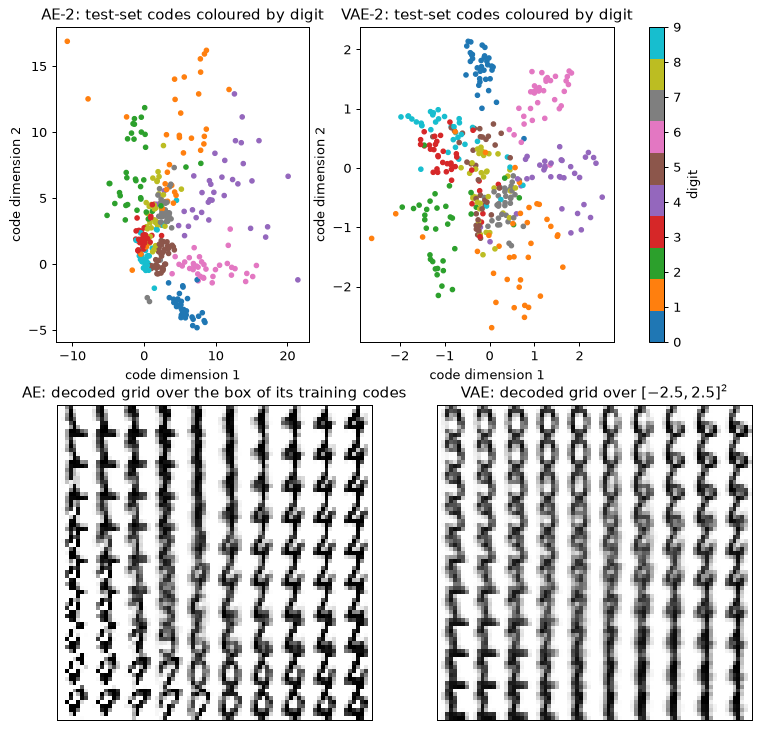
The autoencoder separates the digits best. The two-dimensional PCA codes are the worst, because a flat projection folds several classes on top of one another. The VAE sits between them, and the scatter shows why: the KL term pulls every cloud toward the origin and toward unit width, so the clusters touch. The decoded grids show what the clusters buy. Every cell of the VAE grid is a plausible digit, and the digits change smoothly across the plane. The autoencoder’s grid has sharper digits near the clusters and smudges or implausible shapes in the gaps, because nothing ever asked the decoder to be sensible there. Neither two-dimensional code comes near the raw pixels: ten classes do not fit in two numbers without loss.
Step 6: samples and an interpolation
Generation from a VAE is two lines: draw \mathbf{z} \sim \mathcal{N}(0, \mathbf{I}) from the prior and decode. An interpolation takes the latent means of two real test images, a ‘1’ and a ‘7’, and decodes eight points on the straight line between them. Because the KL term has made the aggregate posterior close to the prior, the line stays in a region the decoder knows.
torch.manual_seed(3)
z = torch.randn(16, 2)
with torch.no_grad():
    samples = torch.sigmoid(vae2.dec(z)).numpy()

i_one = int(np.where(y_te == 1)[0][0])
i_seven = int(np.where(y_te == 7)[0][0])
mu_ends = codes_vae(vae2, Xte_t[[i_one, i_seven]])
alphas = np.linspace(0, 1, 8, dtype=np.float32)[:, None]
z_path = torch.from_numpy((1 - alphas) * mu_ends[0] + alphas * mu_ends[1])
with torch.no_grad():
    path = torch.sigmoid(vae2.dec(z_path)).numpy()
print("latent means of the two ends:", np.round(mu_ends.astype(float), 2).tolist())

fig, axes = plt.subplots(1, 2, figsize=(11, 3.6), gridspec_kw={"width_ratios": [1, 2]})
axes[0].imshow(tile(samples, 4, 4), cmap="gray_r")
axes[0].set_title("16 samples, $z \\sim N(0, I)$")
axes[1].imshow(tile(path, 1, 8), cmap="gray_r")
axes[1].set_title("interpolation from a test '1' to a test '7' (8 steps)")
for ax in axes:
    ax.set_xticks([])
    ax.set_yticks([])
plt.show()
latent means of the two ends: [[-2.09, -0.77], [0.24, -0.33]]
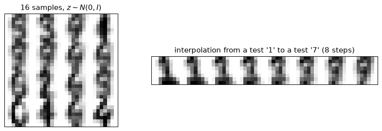
At 8×8 pixels the samples are coarse, and all are soft: the decoder outputs the average of the images consistent with a code (Section 3, blurry samples). Look for digit-like strokes rather than noise; some samples are ambiguous blends of two classes, as the overlap in the scatter predicts. The interpolation changes shape step by step instead of fading one image out and the other in. A pixel-space blend of a ‘1’ and a ‘7’ would be two faint images superimposed. This is the practical meaning of a smooth latent space.
Step 7: causing posterior collapse on purpose
Now the code size is d_z = 8, and the KL weight is varied: \beta = 0.5, 1 and 4. For each model the lab prints the total KL, the KL per dimension, the reconstruction term and the number of active units, the dimensions j for which the variance over the test set of the mean code \mu_j(\mathbf{x}) exceeds 0.01. A fourth model uses the loss of the compact class in Section 3, a summed squared error, which is a Gaussian decoder with \sigma_x^2 = 1/2. Its reconstruction term is on another scale, so only its KL and its active units are comparable with the others.
def active_units(model, data, threshold=0.01):
    with torch.no_grad():
        mu = model.encode(data)[0]
    return int((mu.var(0) > threshold).sum())


runs = {}
settings = [("beta=0.5", 0.5, False), ("beta=1", 1.0, False), ("beta=4", 4.0, False),
            ("beta=1, squared error", 1.0, True)]
for name, beta, gaussian in settings:
    torch.manual_seed(0)
    model = train(VAE(d_z=8, beta=beta, gaussian=gaussian), Xtr_t, vae_loss)
    _, recon, kl, kl_dim = vae_report(model, Xte_t)
    runs[name] = (model, kl_dim)
    print(f"{name:22s} KL {kl:5.2f}  active {active_units(model, Xte_t)}  "
          f"reconstruction {recon:5.1f}")
    print(f"{'':22s} KL per dim {np.round(kl_dim, 2)}")

fig, axes = plt.subplots(1, 4, figsize=(13, 3.2), sharey=True)
for ax, (name, (model, kl_dim)) in zip(axes, runs.items()):
    ax.bar(range(8), kl_dim)
    ax.set_title(name)
    ax.set_xlabel("latent dimension")
axes[0].set_ylabel("KL per dimension (nats)")
plt.show()
beta=0.5               KL  6.51  active 8  reconstruction  18.9
                       KL per dim [1.21 0.9  0.46 1.25 0.42 0.38 0.69 1.2 ]
beta=1                 KL  3.57  active 6  reconstruction  21.0
                       KL per dim [0.84 0.53 0.   0.91 0.   0.01 0.37 0.9 ]
beta=4                 KL  0.00  active 0  reconstruction  27.2
                       KL per dim [0. 0. 0. 0. 0. 0. 0. 0.]
beta=1, squared error  KL  0.48  active 3  reconstruction   4.3
                       KL per dim [0.1  0.   0.   0.21 0.16 0.   0.   0.  ]
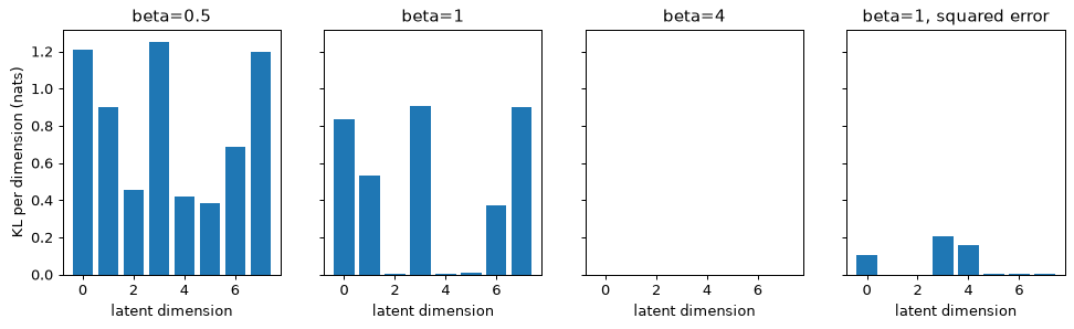
The KL weight sets how much information the code may carry. At \beta = 0.5 the code carries 6.5 nats and all eight dimensions are used. At \beta = 1, the true ELBO, it carries 3.6 nats and five dimensions hold nearly all of it (3.55 of the 3.57 nats); the other three sit near the prior, and one of them still varies a little with the input, which is why six units count as active. At \beta = 4 every dimension has a KL of zero: the encoder outputs the prior for every image and the decoder produces one average digit, whatever \mathbf{z} is. This is posterior collapse, and here it is not a training accident. The objective itself prefers it: the reconstruction gain from using the code is smaller than four times its KL cost (Section 3 works through the numbers). The squared-error loss collapses most of the dimensions for the same reason in a milder form, because \sigma_x^2 = 1/2 makes reconstruction cheap to give up.
Diagnose collapse from the KL per dimension, as above, and not from the loss: a collapsed model has a perfectly steady loss.
Step 8: an anomaly detector with an honest threshold
The last task is the use of Section 2. The detector is trained only on normal data, the digits 0 to 8, and the 9s play the part of an unforeseen fault. The training digits are split again: 80% to fit the autoencoder and 20% held out as a validation set of normal data, from which the threshold is read. The threshold is the 95th percentile of the validation errors, so the false-alarm rate on normal data should be close to 5% by construction. The detection rate on the 9s is not set by anything; it is measured. The test set is used once, at the end.
The baseline is the monitor an engineer would build first: PCA with 8 components fitted on the same normal data, scored by the Q statistic, the squared reconstruction error, with its own 95th-percentile threshold from the same validation set.
normal_tr = y_tr <= 8
X_norm = X_tr[normal_tr]
X_fit, X_val = train_test_split(X_norm, test_size=0.2, random_state=0)
X_test_normal = X_te[y_te <= 8]
X_test_nine = X_te[y_te == 9]
print(f"fit {len(X_fit)}, validation {len(X_val)}, test normal {len(X_test_normal)}, "
      f"test nines {len(X_test_nine)}")

torch.manual_seed(0)
ae_norm = train(AutoEncoder(d_z=8), torch.from_numpy(X_fit), ae_loss)
pca_norm = PCA(n_components=8).fit(X_fit)


def error_ae(data):
    with torch.no_grad():
        t = torch.from_numpy(data)
        return ((ae_norm(t) - t) ** 2).mean(1).numpy()


def error_pca(data):
    return ((pca_norm.inverse_transform(pca_norm.transform(data)) - data) ** 2).mean(1)


results = {}
for name, score in (("autoencoder", error_ae), ("PCA Q statistic", error_pca)):
    threshold = np.percentile(score(X_val), 95)
    e_norm, e_nine = score(X_test_normal), score(X_test_nine)
    auc = roc_auc_score(np.r_[np.zeros(len(e_norm)), np.ones(len(e_nine))],
                        np.r_[e_norm, e_nine])
    results[name] = (e_norm, e_nine, threshold)
    print(f"{name:16s} threshold {threshold:.4f}  false alarms {np.mean(e_norm > threshold):.3f}"
          f"  9s detected {np.mean(e_nine > threshold):.3f}  AUC {auc:.3f}")

fig, axes = plt.subplots(1, 2, figsize=(11, 3.8), sharey=True)
for ax, (name, (e_norm, e_nine, threshold)) in zip(axes, results.items()):
    bins = np.linspace(0, max(e_norm.max(), e_nine.max()), 40)
    ax.hist(e_norm, bins=bins, alpha=0.6, label="normal test digits 0-8")
    ax.hist(e_nine, bins=bins, alpha=0.6, label="test 9s (anomalies)")
    ax.axvline(threshold, color="k", linestyle="--", label="95th-percentile threshold")
    ax.set_title(name)
    ax.set_xlabel("reconstruction error (MSE per pixel)")
axes[0].set_ylabel("number of test images")
axes[0].legend()
plt.show()
fit 1034, validation 259, test normal 324, test nines 36
autoencoder      threshold 0.0261  false alarms 0.040  9s detected 0.583  AUC 0.952
PCA Q statistic  threshold 0.0395  false alarms 0.077  9s detected 0.222  AUC 0.791
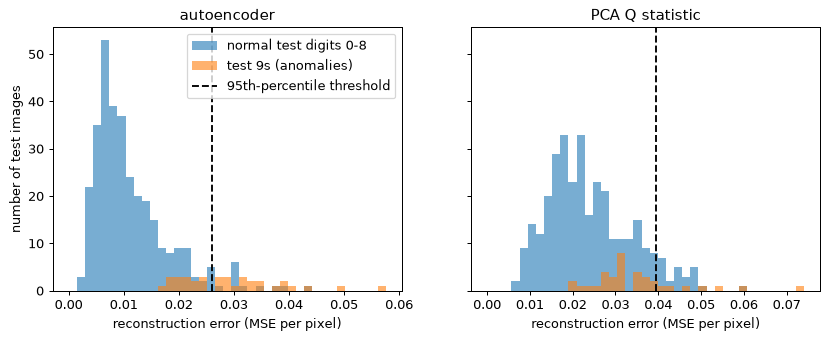
Three things are read from this table, in order. The false-alarm rate on normal test digits is close to the 5% the threshold was set for, which confirms that the validation split did its job (with only 324 normal test images a gap of a point or two is noise). The detection rate is a property of the anomaly, not of the threshold: only about 58% of the 9s are caught, even though the AUC is 0.95. An AUC averages over every threshold, including ones nobody would run, and says nothing about the one you chose. And the PCA monitor is clearly worse, which is the comparison that justifies the network. The histogram shows the overlap that causes the misses: many 9s have errors inside the normal range because they resemble digits the model reconstructs well.
If you had chosen the threshold on the test errors, to catch more 9s, the reported detection rate would be an artefact of the choice. Choose on validation data, report on test data.
What you should see
- The autoencoder beats PCA at equal code size, by about 30% at d_z = 2 and by more than a factor of two at d_z = 8, because digits lie on a curved manifold.
- The VAE’s two-dimensional codes overlap more than the autoencoder’s (5-NN accuracy about 0.75 against 0.84), because the KL term pulls every code toward \mathcal{N}(0, \mathbf{I}). In exchange every point of the VAE’s grid decodes to a plausible digit, while the autoencoder’s grid has implausible regions between clusters.
- The KL weight controls collapse. At \beta = 4 every dimension has a KL of 0.00 and the decoder outputs an average digit. The summed-squared-error loss, with \sigma_x^2 = 1/2, leaves only about three of eight dimensions active.
- An AUC of 0.95 does not mean 95% detection. At a threshold that gives about 5% false alarms, about 58% of the 9s are caught. The PCA monitor is worse on both counts.
Try this
- KL warm-up. Ramp \beta linearly from 0 to 1 over the first 50 epochs in the d_z = 8 VAE and count active units: expect them to rise from 6 to 8, the two extra carrying little KL (a run of this extension gave 8 active units and a KL of 3.48 nats, the two new dimensions at 0.01 and 0.04). Ramp to \beta = 4 instead and the model still collapses (KL 0.01, no active units). Warm-up repairs collapse that comes from the path of optimisation, not collapse that is the optimum of the objective.
- Clusters in two dimensions. Generate 3,000 points from three 2D Gaussian clusters with means (-2, 0), (2, 0), (0, 2.5) and standard deviation 0.3. Train the VAE with d_x = 2, d_z = 2 and a Gaussian decoder, and plot the latent means coloured by cluster. Then set d_z = 1 and see whether the clusters stay apart.
- Another anomaly. Hold out the digit 8 instead of 9, then the digit 0, with the same threshold rule. Detection rises sharply for one of them. Which digits are hard anomalies for this model, and why does it depend on which digits remain in the normal class?
Lab 2 — A diffusion model on two moons, with classifier-free guidance
Goal. You implement the pieces of Section 5 and Section 6 on data small enough to
look at: the forward noising process with a cosine schedule, a noise-prediction network trained
with the simple loss, ancestral sampling from the reverse process, classifier-free guidance, and
the deterministic DDIM sampler with fewer steps. The data are the two interleaved moons of
make_moons, a 2D distribution whose quality can be measured with nearest-neighbour distances
instead of judged by eye. You will see the structure of a sample appear late in the reverse
process, see guidance trade diversity for fidelity, and see quality fall as steps are removed.
The data are synthetic, there is no download, and the lab runs in about two minutes on a laptop
CPU (105 s in the run shown): the network has 37,858 parameters, and training is 95 s of that. Set
QUICK = True in the first block to train for 8,000 steps instead of 20,000 and finish in about
a minute. Printed numbers may differ from
yours in the last digits.
Step 1: the noise schedule, and why it is capped
The forward process of Section 5 turns data into noise in T steps. With \alpha_t = 1 - \beta_t and \bar\alpha_t = \prod_{s \le t}\alpha_s, a noised point is \mathbf{x}_t = \sqrt{\bar\alpha_t}\,\mathbf{x}_0 + \sqrt{1 - \bar\alpha_t}\,\boldsymbol\epsilon. The schedule is the cosine schedule of Nichol and Dhariwal: \bar\alpha_t is proportional to \cos^2\!\big(\tfrac{t/T + s}{1 + s}\cdot\tfrac{\pi}{2}\big) with s = 0.008, normalised so that \bar\alpha_0 = 1, and each \beta_t = 1 - \bar\alpha_t/\bar\alpha_{t-1}. This lab uses T = 200, not the 1,000 of the paper, because two moons need far less.
The one change from the paper is a cap: \beta_t \le 0.5 instead of 0.999. The uncapped schedule ends with \beta_T = 1 and \bar\alpha_T = 0. The reverse step divides by \sqrt{\alpha_t}, so the last step, where \alpha_T = 1 - \beta_T is tiny, multiplies whatever error the network made by 1/\sqrt{\alpha_T}. With \beta_T = 0.999 that is 31.6, with the cap 1.41. The first block prints the factor for both so that you can see the size of the effect. The cap leaves \bar\alpha_T at a small positive number, and the sampler starts from \mathcal{N}(0, \mathbf{I}), which is then a very slightly wrong starting distribution; for this data the error is invisible.
import time

import matplotlib.pyplot as plt
import numpy as np
import torch
import torch.nn as nn
import torch.nn.functional as F
from sklearn.datasets import make_moons
from sklearn.neighbors import KNeighborsClassifier, NearestNeighbors

np.random.seed(0)
torch.manual_seed(0)
torch.set_num_threads(2)

QUICK = False  # True: 8,000 training steps instead of 20,000
T = 200


def cosine_alpha_bar(T, s=0.008):
    """alpha-bar_t for t = 0..T from the cosine schedule, with alpha-bar_0 = 1."""
    t = np.arange(T + 1) / T
    f = np.cos((t + s) / (1 + s) * np.pi / 2) ** 2
    return f / f[0]


ab_cos = cosine_alpha_bar(T)
beta_uncapped = 1 - ab_cos[1:] / ab_cos[:-1]  # entry t-1 is beta_t
beta = np.minimum(beta_uncapped, 0.5)  # the cap
alpha = 1 - beta
alpha_bar = np.concatenate([[1.0], np.cumprod(alpha)])  # alpha_bar[t] for t = 0..T

print(f"alpha_bar_1 {alpha_bar[1]:.5f}  alpha_bar_100 {alpha_bar[100]:.4f}  "
      f"alpha_bar_200 {alpha_bar[200]:.2e}")
print("last three uncapped betas:", np.round(beta_uncapped[-3:], 4))
print(f"error factor 1/sqrt(alpha_T): capped {1 / np.sqrt(alpha[-1]):.2f}, "
      f"beta_T = 0.999 gives {1 / np.sqrt(1 - 0.999):.1f}")

plt.figure(figsize=(6, 3.5))
plt.plot(np.arange(T + 1), alpha_bar)
plt.xlabel("step t")
plt.ylabel(r"$\bar\alpha_t$ (fraction of signal variance left)")
plt.title("Cosine noise schedule, T = 200, beta capped at 0.5")
plt.show()
alpha_bar_1 0.99975  alpha_bar_100 0.4938  alpha_bar_200 6.83e-05
last three uncapped betas: [0.5555 0.75   1.    ]
error factor 1/sqrt(alpha_T): capped 1.41, beta_T = 0.999 gives 31.6
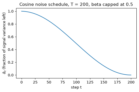
The signal falls slowly at first and faster later: 0.85 of its variance is left at t = 50, half at t = 100 and 0.14 at t = 150, and the last fifty steps take the rest to nearly zero. The cosine schedule is chosen for this shape, which spends many steps at moderate noise levels, where the structure of the data is partly visible, instead of burning through them. Training and sampling below use the capped values throughout, so the forward and reverse processes agree with each other.
Step 2: the forward process, drawn
The closed form lets you jump straight to any step. One fixed noise draw \boldsymbol\epsilon per point is reused at every t, so that each point slides along a single straight line from its origin toward noise and the panels are comparable. The data are standardised first, to zero mean and unit variance in each coordinate, so that the end state \mathcal{N}(0, \mathbf{I}) has the same scale as the data. Standardisation uses the mean and standard deviation of the training set itself; the same numbers will be applied to the evaluation set.
X_raw, y_raw = make_moons(n_samples=10000, noise=0.05, random_state=0)
mean, std = X_raw.mean(0), X_raw.std(0)
data = torch.tensor((X_raw - mean) / std, dtype=torch.float32)
labels = torch.tensor(y_raw)
X_ref_raw, y_ref = make_moons(n_samples=5000, noise=0.05, random_state=1)
X_ref = ((X_ref_raw - mean) / std).astype(np.float32)  # reference set for evaluation
print("standardised data: mean", np.round(data.mean(0).numpy(), 3),
      " std", np.round(data.std(0).numpy(), 3))

ab = torch.tensor(alpha_bar, dtype=torch.float32)


def noise_to(x0, t, eps):
    """Closed-form forward process: x_t from x_0 in one step (t is a tensor of step indices)."""
    a = ab[t][:, None]
    return a.sqrt() * x0 + (1 - a).sqrt() * eps


eps_fixed = torch.randn(1500, 2)
x0_show, y_show = data[:1500], labels[:1500].numpy()
steps = (0, 50, 100, 150, 175, 200)
fig, axes = plt.subplots(1, 6, figsize=(16, 2.9), sharex=True, sharey=True)
for ax, t in zip(axes, steps):
    xt = noise_to(x0_show, torch.full((1500,), t), eps_fixed).numpy()
    ax.scatter(xt[:, 0], xt[:, 1], c=y_show, cmap="coolwarm", s=3)
    ax.set_title(f"t = {t}, $\\bar\\alpha_t$ = {alpha_bar[t]:.3f}")
    ax.set_xlabel("$x_1$")
axes[0].set_ylabel("$x_2$")
plt.show()
standardised data: mean [-0. -0.] std [1. 1.]
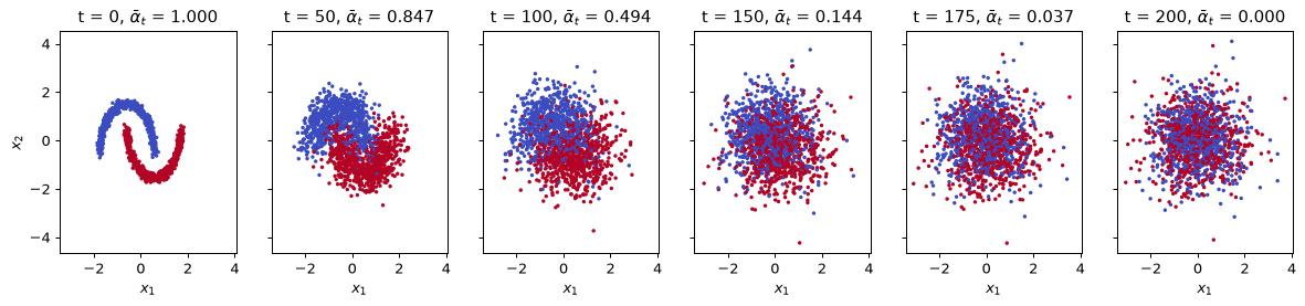
By t = 50 the thin crescents have already become two broad overlapping clouds, one per moon. By t = 100 they are two heavily overlapping blobs, and from t = 150 on the two classes are mixed and only a Gaussian cloud remains. The fine geometry of the data, the curve of the crescents, is destroyed early in the forward process. The reverse process must put it back, which is the first hint of the late-structure observation of Step 5.
Step 3: the denoising network
The network \boldsymbol\epsilon_\theta(\mathbf{x}_t, t, c) predicts the noise that was added. It needs to know the step t, because the right answer depends on how noisy the input is, and the condition c: the moon label 0 or 1, or a third value, null, standing for “no condition”. The null value is what makes classifier-free guidance possible in Step 6, because the same network then gives both a conditional and an unconditional prediction.
The step is encoded as a 32-dimensional sinusoidal embedding, as in the transformer, and the condition by a learned 32-dimensional embedding of three entries. The two embeddings are added, and the sum is concatenated to the 2 coordinates of \mathbf{x}_t. Three hidden layers of 128 units with SiLU activations and a linear output of 2 numbers follow. The parameter count is 34 \cdot 128 + 128 + 2(128 \cdot 128 + 128) + 128 \cdot 2 + 2 + 3 \cdot 32 = 37{,}858.
def time_embedding(t, dim=32):
    """Sinusoidal embedding of the step index, shape (B, dim)."""
    freqs = torch.exp(-np.log(10000.0) * torch.arange(dim // 2) / (dim // 2))
    angles = t.float()[:, None] * freqs[None, :]
    return torch.cat([angles.sin(), angles.cos()], dim=-1)


NULL = 2  # condition index meaning "no condition"


class Denoiser(nn.Module):
    def __init__(self, hidden=128, d_emb=32):
        super().__init__()
        self.cond_emb = nn.Embedding(3, d_emb)  # moon 0, moon 1, null
        self.net = nn.Sequential(
            nn.Linear(2 + d_emb, hidden), nn.SiLU(),
            nn.Linear(hidden, hidden), nn.SiLU(),
            nn.Linear(hidden, hidden), nn.SiLU(),
            nn.Linear(hidden, 2),
        )

    def forward(self, x, t, c):
        emb = time_embedding(t) + self.cond_emb(c)
        return self.net(torch.cat([x, emb], dim=-1))


model = Denoiser()
print("parameters:", sum(p.numel() for p in model.parameters()))
parameters: 37858
Step 4: training with the simple loss
Each training step draws a batch of 512 clean points, a step t uniform on \{1, \dots, 200\} for
each, and noise \boldsymbol\epsilon; forms \mathbf{x}_t; and minimises the mean squared error
between \boldsymbol\epsilon and \boldsymbol\epsilon_\theta(\mathbf{x}_t, t, c). This is the
objective of Section 5, a plain regression. With probability 0.2 the condition is replaced by
NULL, so that one network learns both the conditional and the unconditional noise. Adam with
learning rate 10^{-3} and cosine decay to zero finishes the run.
The loss does not fall to zero and should not: the noise is random, and the network can only predict the part of it that \mathbf{x}_t and t reveal. At small t, \mathbf{x}_t is nearly \mathbf{x}_0 and the noise is almost unrecoverable from one point. At large t the noise is almost all there is of \mathbf{x}_t, and the task is easy. The printed loss is therefore an average over very different difficulties, and a flat curve says little about sample quality.
n_steps = 8000 if QUICK else 20000
opt = torch.optim.Adam(model.parameters(), lr=1e-3)
sched = torch.optim.lr_scheduler.CosineAnnealingLR(opt, T_max=n_steps)
torch.manual_seed(0)
t0 = time.time()
fifth = n_steps // 5
running = []
for step in range(1, n_steps + 1):
    idx = torch.randint(0, len(data), (512,))
    x0, c = data[idx], labels[idx].clone()
    c[torch.rand(512) < 0.2] = NULL  # condition dropout for classifier-free guidance
    t = torch.randint(1, T + 1, (512,))
    eps = torch.randn(512, 2)
    loss = F.mse_loss(model(noise_to(x0, t, eps), t, c), eps)
    opt.zero_grad()
    loss.backward()
    opt.step()
    sched.step()
    running.append(loss.item())
    if step % fifth == 0:
        print(f"step {step:6d}  mean loss over the last {fifth} steps "
              f"{np.mean(running[-fifth:]):.4f}")
print(f"training time {time.time() - t0:.0f} s")
step   4000  mean loss over the last 4000 steps 0.3646
step   8000  mean loss over the last 4000 steps 0.3324
step  12000  mean loss over the last 4000 steps 0.3294
step  16000  mean loss over the last 4000 steps 0.3277
step  20000  mean loss over the last 4000 steps 0.3260
training time 95 s
The loss is 0.36 over the first fifth and settles near 0.33 afterwards. That is an average over all noise levels of an error that cannot go below the noise floor, so the curve is nearly flat long before the samples stop improving. A loss of 0.33 does not say whether the moons will be sharp; the nearest-neighbour measurements of the next steps do. The training time depends on the machine, and on a busy one it can be twice the minute and a half of a quiet laptop.
Step 5: ancestral sampling, and what it produces
Sampling starts from \mathbf{x}_T \sim \mathcal{N}(0, \mathbf{I}) and applies, for t = T, \dots, 1, the update of Ho et al. (Algorithm 2):
with \mathbf{z} = 0 at the last step. The first factor removes the predicted noise and rescales; the second adds back a smaller amount of fresh noise, with variance \beta_t, which keeps the chain a proper sample from the reverse process rather than a deterministic slide. The function below takes a condition and a guidance scale w; this step uses the null condition, so w plays no role, and Step 6 uses both.
Samples are scored with nearest-neighbour distances, in standardised units. The mean distance from each sample to its nearest point of a 5,000-point reference set is a precision-like quantity: small when samples lie on the moons. The mean distance from each reference point to its nearest sample is a recall-like quantity: small when the samples cover every part of the moons. Two yardsticks calibrate them: 2,000 fresh draws from the true distribution, which is the best any sampler could do, and 2,000 draws from \mathcal{N}(0, \mathbf{I}), which is the starting point.
@torch.no_grad()
def eps_hat(x, t_int, c, w):
    """Noise prediction; with a condition c in {0, 1}, classifier-free guidance of scale w."""
    t = torch.full((len(x),), t_int, dtype=torch.long)
    e_null = model(x, t, torch.full((len(x),), NULL))
    if c == NULL:
        return e_null
    e_cond = model(x, t, torch.full((len(x),), c))
    return e_null + w * (e_cond - e_null)


beta_t, alpha_t, ab_t = (torch.tensor(a, dtype=torch.float32) for a in (beta, alpha, alpha_bar))


@torch.no_grad()
def ancestral(n, c=NULL, w=0.0, seed=0, snapshots=()):
    """Ho et al. Algorithm 2. Returns x_0 and {t: x_t before the update at step t}."""
    gen = torch.Generator().manual_seed(seed)
    x = torch.randn(n, 2, generator=gen)
    snaps = {}
    for t in range(T, 0, -1):
        if t in snapshots:
            snaps[t] = x.clone().numpy()
        e = eps_hat(x, t, c, w)
        x = (x - beta_t[t - 1] / (1 - ab_t[t]).sqrt() * e) / alpha_t[t - 1].sqrt()
        if t > 1:
            x = x + beta_t[t - 1].sqrt() * torch.randn(n, 2, generator=gen)
    return x.numpy(), snaps


def nn_dist(a, b):
    """Mean distance from each row of a to its nearest row of b."""
    return float(NearestNeighbors(n_neighbors=1).fit(b).kneighbors(a)[0].mean())


fresh_raw, _ = make_moons(n_samples=2000, noise=0.05, random_state=2)
fresh = ((fresh_raw - mean) / std).astype(np.float32)
noise_pts = np.random.default_rng(0).standard_normal((2000, 2)).astype(np.float32)
for name, pts in (("fresh data", fresh), ("N(0, I) noise", noise_pts)):
    print(f"{name:14s} precision-like {nn_dist(pts, X_ref):.3f}   "
          f"recall-like {nn_dist(X_ref, pts):.3f}")

t0 = time.time()
snap_steps = (200, 150, 100, 50, 20, 5)
x_gen, snaps = ancestral(2000, snapshots=snap_steps)
print(f"unconditional samples  precision-like {nn_dist(x_gen, X_ref):.3f}   "
      f"recall-like {nn_dist(X_ref, x_gen):.3f}   ({time.time() - t0:.1f} s)")
print("precision-like distance of x_t at t =", snap_steps, ":",
      [round(nn_dist(snaps[t], X_ref), 3) for t in snap_steps])

fig, axes = plt.subplots(1, 7, figsize=(18, 2.8), sharex=True, sharey=True)
for ax, t in zip(axes, snap_steps):
    ax.scatter(snaps[t][:, 0], snaps[t][:, 1], s=2)
    ax.set_title(f"$x_t$ at t = {t}")
    ax.set_xlabel("$x_1$")
axes[-1].scatter(x_gen[:, 0], x_gen[:, 1], s=2, color="tab:green")
axes[-1].set_title("final sample $x_0$")
axes[-1].set_xlabel("$x_1$")
axes[0].set_ylabel("$x_2$")
plt.show()
fresh data     precision-like 0.013   recall-like 0.021
N(0, I) noise  precision-like 0.242   recall-like 0.051
unconditional samples  precision-like 0.022   recall-like 0.022   (0.5 s)
precision-like distance of x_t at t = (200, 150, 100, 50, 20, 5) : [0.246, 0.234, 0.212, 0.134, 0.057, 0.027]
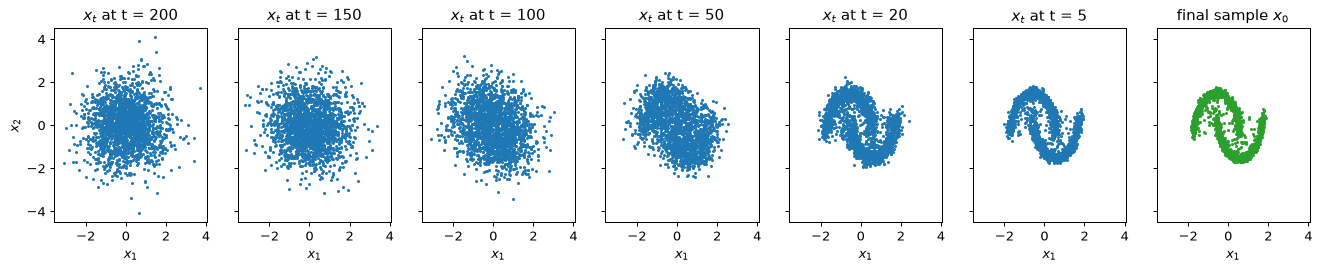
Read the two yardsticks first. Fresh data sit at about 0.013 from the reference set and the reference is about 0.021 from them, which are the floors set by sample size and by the noise of the moons: no sampler can beat them. Noise sits at 0.24 and 0.05. The model’s samples land close to the floor on both counts: they are on the moons, and they cover both of them. The six snapshots show where this happens. The precision-like distance of \mathbf{x}_t is still about 0.25 at t = 200, as for pure noise, falls only slowly until t = 100 (0.212), is 0.134 at t = 50, and drops to the final 0.022 within the last fifty steps. Structure appears late: the snapshots at t = 100 and t = 50 are shapeless blobs with a hint of the two moons, and the crescents sharpen only between t = 50 and t = 5. That is why the last steps matter most for quality, and why removing steps is costly in Step 7.
With QUICK = True expect a precision-like distance of about 0.04 and a recall-like distance of
about 0.025 (a run with QUICK = True gave 0.039 and 0.025): visibly fuzzier moons, with stray points near the moons. The model has been trained for fewer steps, and every step it
takes in the reverse chain compounds its error.
Step 6: classifier-free guidance
A conditional model samples from p(\mathbf{x} \mid c). Guidance sharpens it. The noise prediction used in the update is
where \varnothing is the null condition. With w = 0 it is the unconditional model; with w = 1 it is the conditional model; with w > 1 it moves further along the direction from “anything” to “class c” than the conditional model alone does. The scale is written here as in the code, w = 1 for the plain conditional model. Ho and Salimans write the same thing with (1 + w), so their w = 0 is this lab’s w = 1.
The block samples 1,000 points of class 0 for w = 0, 1, 3, 7. A 15-nearest-neighbour classifier fitted on the labelled reference set says which moon each sample landed on; the fraction on moon 0 measures how well the condition was obeyed. The precision-like distance uses all reference points. The recall-like distance uses only the reference points of class 0, because that is the distribution being sampled.
knn = KNeighborsClassifier(15).fit(X_ref, y_ref)
ref_class0 = X_ref[y_ref == 0]
guided = {}
for w in (0, 1, 3, 7):
    x_w, _ = ancestral(1000, c=0, w=float(w), seed=10 + w)
    guided[w] = x_w
    frac = float((knn.predict(x_w) == 0).mean())
    print(f"w = {w}: fraction on moon 0 {frac:.2f}   precision-like {nn_dist(x_w, X_ref):.3f}"
          f"   recall-like (class-0 points) {nn_dist(ref_class0, x_w):.3f}")

fig, axes = plt.subplots(1, 4, figsize=(15, 3.4), sharex=True, sharey=True)
for ax, w in zip(axes, guided):
    ax.scatter(X_ref[:, 0], X_ref[:, 1], s=1, color="lightgrey")
    ax.scatter(guided[w][:, 0], guided[w][:, 1], s=3, color="tab:red")
    ax.set_title(f"class 0, guidance w = {w}")
    ax.set_xlabel("$x_1$")
axes[0].set_ylabel("$x_2$")
plt.show()
w = 0: fraction on moon 0 0.50   precision-like 0.023   recall-like (class-0 points) 0.032
w = 1: fraction on moon 0 1.00   precision-like 0.014   recall-like (class-0 points) 0.021
w = 3: fraction on moon 0 1.00   precision-like 0.013   recall-like (class-0 points) 0.029
w = 7: fraction on moon 0 1.00   precision-like 0.020   recall-like (class-0 points) 0.043
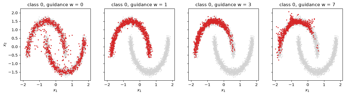
With w = 0 the condition is ignored and half the samples fall on each moon: the unconditional model. Its recall-like distance to the class-0 points is high (0.032) because only half of its samples are near them. At w = 1 every sample is on the requested moon and the recall-like distance is at its best, 0.021. The fraction on the moon cannot improve beyond 1.00, but the other numbers keep moving. The recall-like distance grows with w (0.029 at w = 3, 0.043 at w = 7), because the samples concentrate on the densest part of the moon and its two tips go unvisited, as the figure shows. At w = 7 the precision-like distance has grown too (0.020 against 0.013 at w = 3), because the stronger push overshoots: some samples leave the moon past its upper left end. This is the trade-off of guidance in its purest form. Fidelity to the condition is bought with diversity, and past some scale it is bought with a worse fit as well.
Step 7: DDIM and the cost of steps
Ancestral sampling takes 200 network evaluations per sample. DDIM (Song et al.) reuses the same trained network with a deterministic update that may skip steps. At each step it first estimates the clean point from the noise prediction,
which inverts the forward formula, and then re-noises it to the next, lower noise level t' with the same predicted noise:
No fresh noise is injected, so the map from \mathbf{x}_T to \mathbf{x}_0 is deterministic. Because the update only needs \bar\alpha_t and \bar\alpha_{t'}, t' need not be t - 1: K evenly spaced steps from 200 to 0 give a K-step sampler with no retraining. The block measures unconditional samples for K = 200, 50, 20, 10, 5, 2, 1, with the time each takes. The K = 1 row is \hat{\mathbf{x}}_0 from one evaluation at t = 200.
@torch.no_grad()
def ddim(n, K, seed=0):
    gen = torch.Generator().manual_seed(seed)
    x = torch.randn(n, 2, generator=gen)
    ts = np.round(np.linspace(T, 0, K + 1)).astype(int)
    for t, t_next in zip(ts[:-1], ts[1:]):
        e = eps_hat(x, int(t), NULL, 0.0)
        x0_hat = (x - (1 - ab_t[t]).sqrt() * e) / ab_t[t].sqrt()
        x = ab_t[t_next].sqrt() * x0_hat + (1 - ab_t[t_next]).sqrt() * e
    return x.numpy()


print("   K  precision-like  recall-like  seconds")
ddim_samples = {}
for K in (200, 50, 20, 10, 5, 2, 1):
    t0 = time.time()
    xs = ddim(2000, K)
    ddim_samples[K] = xs
    print(f"{K:4d}  {nn_dist(xs, X_ref):13.3f}  {nn_dist(X_ref, xs):11.3f}  {time.time() - t0:7.2f}")

fig, axes = plt.subplots(1, 4, figsize=(14, 3.3), sharex=True, sharey=True)
for ax, K in zip(axes, (50, 10, 5, 1)):
    xs = ddim_samples[K]
    outside = int((np.abs(xs).max(1) > 3).sum())
    ax.scatter(xs[:, 0], xs[:, 1], s=2)
    ax.set_xlim(-3, 3)
    ax.set_ylim(-3, 3)
    ax.set_title(f"DDIM, K = {K} steps ({outside} of 2000 outside the box)")
    ax.set_xlabel("$x_1$")
axes[0].set_ylabel("$x_2$")
plt.show()
   K  precision-like  recall-like  seconds
 200          0.022        0.023     0.84
  50          0.022        0.024     0.21
  20          0.025        0.029     0.12
  10          0.035        0.042     0.07
   5          0.046        0.067     0.03
   2          0.152        0.120     0.02
   1          1.714        0.142     0.02
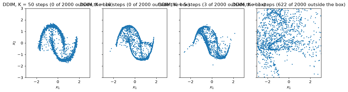
Twenty to fifty DDIM steps give samples close to the 200-step ancestral sampler’s, with a quarter to a tenth of its network evaluations; the time column falls almost in proportion to K. Below about ten steps quality falls quickly. One step is a different kind of failure. At t = 200 the signal weight is \sqrt{\bar\alpha_{200}} = 0.008, so the estimate \hat{\mathbf{x}}_0 divides the network’s output by 0.008, a factor of 121, and any error in \boldsymbol\epsilon_\theta is blown up by that factor. The one-step samples therefore scatter far outside the data, a precision-like distance of well over 1, even though their recall-like distance is only 0.14: the data region is covered, by a cloud that also covers a great deal more. The cost of diffusion is its number of steps, and what the steps buy is the gradual commitment to structure that you saw in Step 5.
What you should see
- Structure appears late in the reverse process. The intermediate samples are shapeless until about t = 50 (precision-like distance 0.134, against 0.246 for noise), and the crescents form between t = 50 and t = 5.
- The unconditional samples are almost as close to the data as fresh data are (about 0.022 against 0.013) and cover both moons (recall-like distance 0.022 against 0.021).
- Guidance trades diversity for fidelity. w = 1 already puts every sample on the requested moon. w = 3 and w = 7 squeeze the samples toward the densest part of the moon, the recall-like distance doubling by w = 7, and at w = 7 the precision-like distance starts to worsen as samples overshoot.
- DDIM with 20 to 50 steps is close to the 200-step ancestral sampler. Below about 10 steps quality falls quickly, and a single step returns a smeared estimate far from the data.
- The cap on \beta_t is a safeguard. With the paper’s cap of 0.999 the first reverse step multiplies the network’s error by 31.6, against 1.41 with the cap at 0.5. Whether that hurts depends on the run: in a prototype made when the module was planned the w = 7 samples diverged (a precision-like distance of 1.34), while a copy of this lab retrained with the 0.999 cap in the current environment gave 0.019 at w = 7, as good as the capped model. The cap removes the risk at no cost.
Try this
- Restore the cap. Set the cap to 0.999 and repeat Step 6. Then keep the 0.999 cap but compute \hat{\mathbf{x}}_0, clip it to [-3, 3], and use the posterior-mean update \tilde\mu_t from \hat{\mathbf{x}}_0 instead. This is how the original implementations survive the uncapped schedule.
- A GAN on the same data. Train the non-saturating GAN of Section 4 (generator and discriminator: MLPs with three hidden layers of 128, Adam with learning rate 10^{-3} and \beta = (0.5, 0.999)) on the same standardised moons for 6,000 steps. Compare its precision-like and recall-like distances with the diffusion model’s. It needs one forward pass per sample; the diffusion model needs 200.
- The linear schedule. Replace the schedule by the linear range of Ho et al., \beta_t from 10^{-4} to 0.02, kept at T = 200, which ends at \bar\alpha_T = 0.13 (a copy of this lab retrained with it gave a precision-like distance of 0.020 and a recall-like distance of 0.022). On these 2D standardised data the damage is small. Explain why two-dimensional standardised data hide a problem that matters for images: what does \bar\alpha_T = 0.13 leave in the starting sample?
Lab 3 — A graph convolutional network from scratch: single points of failure in fault trees
Goal. You build message passing from the edge list up, in about thirty lines, and use it on a task whose answer is known exactly: finding the single points of failure of a fault tree, the basic events whose failure alone brings down the top event. You write a generator for random fault trees and a labeller for the ground truth, measure two baselines that the models must beat, train graph convolutional networks (Section 7) of increasing depth, and watch the depth limits of Section 8 happen: accuracy by distance from the top, over-smoothing measured without any training, and the repair by residual connections. Last, you replace the symmetric adjacency by a direction-aware layer, which uses the one piece of structure the plain GCN throws away. The data are synthetic and the lab uses no graph library; it runs in about three minutes on a laptop CPU (168 s in the run shown), and needs NumPy, PyTorch and matplotlib. It runs PyTorch on one thread: on several, the scatter-adds of message passing sum in an order that changes from run to run, and so do the accuracies. Even on one thread they move by a point or two with the PyTorch version, so read them as phenomena, not as digits.
Step 1: a fault-tree generator and its labels
A fault tree has gates (OR: the output fails if any input fails; AND: only if all inputs fail) and basic events, the leaves. A basic event is a single point of failure if every gate on its path to the top event is an OR: then its failure alone propagates all the way up. One AND gate anywhere on the path means the other inputs of that gate must fail too.
The generator follows a fixed recipe. The top event is a gate, OR with probability 0.6 and AND otherwise. Every gate has two to four inputs, uniformly. An input of a gate at depth 0 or 1 is itself a gate with probability 0.6, at depth 2 with probability 0.35, and a gate at depth 3 has only basic events as inputs, so no tree is deeper than four levels below the top. Every non-top gate is an OR with probability 0.6. Each node has four features: a one-hot encoding of its type (OR, AND, basic event) and a flag that marks the top event. Gates are not scored; the label of a basic event is 1 for a single point of failure.
The lab generates 300 trees from one seeded generator, uses 200 for training and 100 for testing, and splits by tree, so that the test trees are new graphs, never nodes of a training tree. Engineering models are used on new models, not on new nodes of an old one (Section 7).
import matplotlib.pyplot as plt
import numpy as np
import torch
import torch.nn as nn
import torch.nn.functional as F

np.random.seed(0)
torch.manual_seed(0)
torch.set_num_threads(1)    # scatter-adds sum in a fixed order only on one thread

OR, AND, BASIC = 0, 1, 2


def make_tree(rng):
    """One random fault tree as arrays: node type, parent index (-1 for the top), depth."""
    types, parent, depth = [], [], []

    def add(kind, par, d):
        types.append(kind)
        parent.append(par)
        depth.append(d)
        return len(types) - 1

    top = add(OR if rng.random() < 0.6 else AND, -1, 0)
    open_gates = [top]
    while open_gates:
        g = open_gates.pop()
        d = depth[g]
        p_gate = 0.6 if d <= 1 else (0.35 if d == 2 else 0.0)
        for _ in range(rng.integers(2, 5)):  # 2 to 4 inputs
            if rng.random() < p_gate:
                open_gates.append(add(OR if rng.random() < 0.6 else AND, g, d + 1))
            else:
                add(BASIC, g, d + 1)
    return {"type": np.array(types), "parent": np.array(parent), "depth": np.array(depth)}


def label_tree(tree):
    """1 for a basic event whose gates up to the top are all OR, 0 for the other basic
    events, -1 for gates (not scored)."""
    label = np.full(len(tree["type"]), -1)
    for v in np.where(tree["type"] == BASIC)[0]:
        label[v], u = 1, tree["parent"][v]
        while u != -1:
            if tree["type"][u] == AND:
                label[v] = 0
            u = tree["parent"][u]
    return label


rng = np.random.default_rng(0)
trees = [make_tree(rng) for _ in range(300)]
for tree in trees:
    tree["label"] = label_tree(tree)
train_trees, test_trees = trees[:200], trees[200:]

sizes = [len(t["type"]) for t in trees]
print(f"nodes per tree: mean {np.mean(sizes):.1f}, min {min(sizes)}, max {max(sizes)}")
for name, group in (("train", train_trees), ("test", test_trees)):
    n_nodes = sum(len(t["type"]) for t in group)
    lab = np.concatenate([t["label"] for t in group])
    dep = np.concatenate([t["depth"] for t in group])
    basic = lab >= 0
    counts = {d: int(((dep == d) & basic).sum()) for d in (1, 2, 3, 4)}
    print(f"{name}: {n_nodes} nodes, {basic.sum()} basic events, "
          f"{lab[basic].mean():.1%} single points of failure; by depth {counts}")
nodes per tree: mean 28.1, min 3, max 92
train: 5579 nodes, 3766 basic events, 22.1% single points of failure; by depth {1: 252, 2: 400, 3: 1169, 4: 1945}
test: 2850 nodes, 1934 basic events, 21.9% single points of failure; by depth {1: 123, 2: 193, 3: 640, 4: 978}
Roughly one basic event in five is a single point of failure, in the training and the test trees alike, so a model that never predicts one is right about four times in five: that is the baseline to beat. Most basic events lie three or four levels below the top, and those are the ones that need the most information to label. Another seed or another draw order gives somewhat different counts (the shares move by a point or two), so do not expect to match these digits from a different generator.
Step 2: check the labeller on a tree you can verify by hand
A labeller that nobody has checked is the commonest source of a wrong benchmark. The cooling-system tree of Section 8 has twelve nodes, and its answer can be read off the diagram. The top event, loss of cooling, is an OR of three inputs: the gate G1, “all pumps fail” (an AND of three pumps), the gate G2, “flow path blocked” (an OR of a valve, a pipe and a gate G3, “both controllers fail”, an AND of two controllers), and the basic event E1, the power supply. The single points of failure are therefore E1 directly, and the valve E5 and the pipe E6 through the OR gate G2. The pumps and controllers sit under an AND.
NAMES = ["TOP", "G1", "G2", "E1", "E2", "E3", "E4", "E5", "E6", "G3", "E7", "E8"]
cooling = {
    "type": np.array([OR, AND, OR, BASIC, BASIC, BASIC, BASIC, BASIC, BASIC, AND, BASIC, BASIC]),
    "parent": np.array([-1, 0, 0, 0, 1, 1, 1, 2, 2, 2, 9, 9]),
}
cooling["depth"] = np.array([0, 1, 1, 1, 2, 2, 2, 2, 2, 2, 3, 3])
cooling["label"] = label_tree(cooling)

found = [NAMES[v] for v in np.where(cooling["label"] == 1)[0]]
print("single points of failure found by the labeller:", found)
assert found == ["E1", "E5", "E6"], "the labeller disagrees with the hand answer"
single points of failure found by the labeller: ['E1', 'E5', 'E6']
The assertion is the point of the step. If it failed, nothing that follows could be believed.
Step 3: two baselines
The accuracy of a model on the test basic events means nothing without the accuracy of something trivial. There are two trivial predictors. Majority class: say “not a single point of failure” for every event. And a rule that sounds right, “the event’s own gate is an OR”: if the gate directly above is an OR, the event looks like a single point of failure. The rule is wrong exactly when an AND gate sits somewhere higher up. Both are computed on the test basic events.
def basic_events(group):
    """Concatenate trees; return labels, own-gate types and depths of the basic events."""
    lab = np.concatenate([t["label"] for t in group])
    own_gate = np.concatenate([t["type"][np.maximum(t["parent"], 0)] for t in group])
    dep = np.concatenate([t["depth"] for t in group])
    m = lab >= 0
    return lab[m], own_gate[m], dep[m]


lab_te, gate_te, dep_te = basic_events(test_trees)
majority = np.mean(lab_te == 0)
own_gate_or = np.mean((gate_te == OR).astype(int) == lab_te)
print(f"majority class (never a single point of failure): {majority:.3f}")
print(f"'own gate is OR' rule:                            {own_gate_or:.3f}")
majority class (never a single point of failure): 0.781
'own gate is OR' rule:                            0.616
The plausible rule is worse than predicting the majority class. Many events whose own gate is an OR have an AND gate higher up, so the rule raises many false alarms. Every model below has to beat both numbers, and a model that beats only the rule has learned nothing about single points of failure.
Step 4: message passing on an edge list
Messages are sent along edges, and the whole layer is one scatter-add. A graph is stored as an edge list: two arrays i and j such that there is an edge from j to i (a message sent from j to i). The GCN’s propagation matrix is \hat{\mathbf{A}} = \tilde{\mathbf{D}}^{-1/2}(\mathbf{A} + \mathbf{I})\tilde{\mathbf{D}}^{-1/2}, so the edge list holds both directions of each tree edge and a self-loop for every node, each with weight 1/\sqrt{\tilde d_i \tilde d_j}, where \tilde d counts the node’s neighbours plus itself. Propagating the features \mathbf{H} is then
out[i] = sum over edges (i, j) of w_ij * H[j]
which index_add_ computes in O(|\mathcal{E}|\,d) time without ever forming an n \times n
matrix. The code builds a Graph for any list of trees (the trees are joined into one big graph
with no edges between them) and checks the edge-list propagation against the dense formula on the
twelve-node tree.
class Graph:
    """A batch of trees as one disconnected graph, with everything a model needs."""

    def __init__(self, group):
        offset, parts = 0, []
        for t in group:
            n = len(t["type"])
            par = np.where(t["parent"] >= 0, t["parent"] + offset, -1)
            parts.append((t["type"], par, t["depth"], t["label"]))
            offset += n
        types = np.concatenate([p[0] for p in parts])
        parent = np.concatenate([p[1] for p in parts])
        self.n = len(types)
        onehot = np.eye(3, dtype=np.float32)[types]
        top_flag = (parent == -1).astype(np.float32)[:, None]
        self.x = torch.from_numpy(np.concatenate([onehot, top_flag], axis=1))
        self.y = torch.from_numpy(np.concatenate([p[3] for p in parts]))
        self.depth = np.concatenate([p[2] for p in parts])
        self.basic = self.y >= 0
        # directed edges child -> parent, used by the direction-aware layer of Step 7
        child_idx = np.where(parent >= 0)[0]
        self.child = torch.from_numpy(child_idx)
        self.par = torch.from_numpy(parent[child_idx])
        n_children = np.bincount(parent[child_idx], minlength=self.n)
        self.n_children = torch.from_numpy(np.maximum(n_children, 1).astype(np.float32))
        # symmetric edge list with self-loops and GCN weights
        loops = np.arange(self.n)
        self.i = torch.from_numpy(np.concatenate([child_idx, parent[child_idx], loops]))
        self.j = torch.from_numpy(np.concatenate([parent[child_idx], child_idx, loops]))
        deg = np.bincount(self.i.numpy(), minlength=self.n).astype(np.float32)  # includes loop
        self.w = torch.from_numpy(1 / np.sqrt(deg[self.i.numpy()] * deg[self.j.numpy()]))


def propagate(g, H):
    """A_hat @ H from the edge list: one scatter-add."""
    return torch.zeros_like(H).index_add_(0, g.i, g.w[:, None] * H[g.j])


g_cool = Graph([cooling])
n = g_cool.n
A = torch.zeros(n, n)
A[g_cool.child, g_cool.par] = 1.0
A = A + A.T + torch.eye(n)  # A + I
d_inv_sqrt = A.sum(1).pow(-0.5)
A_hat_dense = d_inv_sqrt[:, None] * A * d_inv_sqrt[None, :]

H = torch.randn(n, 5)
diff = (propagate(g_cool, H) - A_hat_dense @ H).abs().max().item()
print(f"edge-list propagation against the dense matrix: max abs difference {diff:.1e}")
print("row sums of A_hat on the cooling tree (not 1: it is not a mean):",
      np.round(A_hat_dense.sum(1).numpy()[:4], 3))

g_train, g_test = Graph(train_trees), Graph(test_trees)
edge-list propagation against the dense matrix: max abs difference 1.2e-07
row sums of A_hat on the cooling tree (not 1: it is not a mean): [1.051 1.372 1.28  0.854]
The two agree to float32 rounding. The row sums are not 1, because the symmetric normalisation weights an edge by both degrees, not by the receiver’s alone; this is what keeps repeated propagation from exploding or shrinking the features (Section 7).
Step 5: GCNs of increasing depth
The model is the GCN of Section 7. A linear layer maps the four features to 32 numbers; L
layers each compute \mathbf{H} \leftarrow \mathrm{ReLU}(\hat{\mathbf{A}}\mathbf{H}\mathbf{W}) with
its own 32 \times 32 matrix; a linear layer maps each node to two class scores. Training is
full-batch, because the whole training set is one graph of a few thousand nodes: Adam with learning
rate 10^{-2}, weight decay 5 \cdot 10^{-4}, 200 epochs, and a cross-entropy loss over the
training basic events only, since gates have no label. The same fit helper trains every model
in this lab. The table shows test accuracy overall and by depth of the event, for
L = 1, 2, 3, 4, 6, 8, 12, 16.
def accuracy_by_depth(pred, g):
    """Accuracy on the basic events, overall and for each depth 1-4."""
    ok = (pred == g.y).numpy()
    out = [ok[g.basic.numpy()].mean()]
    for d in (1, 2, 3, 4):
        out.append(ok[g.basic.numpy() & (g.depth == d)].mean())
    return np.array(out)


def fit(model, g, epochs=200, lr=1e-2, weight_decay=5e-4):
    opt = torch.optim.Adam(model.parameters(), lr=lr, weight_decay=weight_decay)
    for _ in range(epochs):
        loss = F.cross_entropy(model(g)[g.basic], g.y[g.basic])
        opt.zero_grad()
        loss.backward()
        opt.step()
    return model


def evaluate(model, g):
    model.eval()
    with torch.no_grad():
        pred = model(g).argmax(1)
    return accuracy_by_depth(pred, g)


class GCN(nn.Module):
    def __init__(self, L, hidden=32, residual=False):
        super().__init__()
        self.inp = nn.Linear(4, hidden)
        self.layers = nn.ModuleList(nn.Linear(hidden, hidden, bias=False) for _ in range(L))
        self.out = nn.Linear(hidden, 2)
        self.residual = residual

    def forward(self, g):
        h = self.inp(g.x)
        for lin in self.layers:
            m = torch.relu(propagate(g, lin(h)))  # ReLU(A_hat H W)
            h = h + m if self.residual else m
        return self.out(h)


gcn_acc = {}
print("  L   overall   depth1   depth2   depth3   depth4")
for L in (1, 2, 3, 4, 6, 8, 12, 16):
    torch.manual_seed(0)
    gcn_acc[L] = evaluate(fit(GCN(L), g_train), g_test)
    print(f"{L:3d}   " + "   ".join(f"{a:.3f} " for a in gcn_acc[L]))
  L   overall   depth1   depth2   depth3   depth4
  1   0.810    1.000    0.663    0.769    0.843
  2   0.832    1.000    0.886    0.769    0.843
  3   0.897    1.000    0.969    0.920    0.854
  4   0.938    1.000    0.964    0.933    0.929
  6   0.937    1.000    0.938    0.923    0.939
  8   0.959    0.984    0.959    0.958    0.956
 12   0.781    0.537    0.663    0.769    0.843
 16   0.781    0.537    0.663    0.769    0.843
Read the table by columns first. Depth-1 events are labelled correctly by every model with at least one layer, and each extra layer unlocks the next depth: the L = 1 model is already perfect at depth 1 but near the majority rate at depths 3 and 4, and at L = 4 every depth is above 0.92. This is the receptive field. A basic event at depth d has the gates at depths 0, \dots, d-1 above it, the topmost d hops away, so a model with L layers cannot see enough to label events deeper than L exactly.
Then read the rows. Accuracy stays near 0.94 at L = 4 and 6 and is best at L = 8 (0.959), because the symmetric layers mix siblings and gates together and extra layers help to separate them again, and then it falls off a cliff. The 12- and 16-layer models score the majority-class accuracy at every depth: they predict “not a single point of failure” for every event. That is not overfitting, and the next step looks at why.
Step 6: over-smoothing, measured without training
Repeated propagation by \hat{\mathbf{A}} makes the features of connected nodes more and more alike (Section 8). To see this without any network, apply \hat{\mathbf{A}}^k to the raw features of the largest test tree and measure the mean cosine similarity over all pairs of nodes: 1 means every node points the same way. No weights are involved, so this is a property of the graph and the normalisation alone.
The remedy tried here is the one from deep networks in general (Module 03, Section 8): a residual connection, \mathbf{H} \leftarrow \mathbf{H} + \mathrm{ReLU}(\hat{\mathbf{A}}\mathbf{H}\mathbf{W}), so that each node keeps its own features alongside the smoothed ones and the gradient has a direct path through 16 layers.
sizes_test = [len(t["type"]) for t in test_trees]
biggest = Graph([test_trees[int(np.argmax(sizes_test))]])
Z = biggest.x.clone()
print(f"largest test tree: {biggest.n} nodes")
curve_k, curve_cos = [], []
for k in range(1, 65):
    Z = propagate(biggest, Z)
    U = F.normalize(Z, dim=1)
    cos = float(((U @ U.T).sum() - biggest.n) / (biggest.n * (biggest.n - 1)))
    curve_k.append(k)
    curve_cos.append(cos)
    if k in (1, 2, 4, 8, 16, 32, 64):
        print(f"k = {k:2d}: mean pairwise cosine similarity of A_hat^k X = {cos:.3f}")

# Is the 16-layer failure underfitting? Compare train and test accuracy, with and without
# residual connections.
for name, residual in (("plain", False), ("residual", True)):
    torch.manual_seed(0)
    model16 = fit(GCN(16, residual=residual), g_train)
    tr_acc, te_acc = evaluate(model16, g_train)[0], evaluate(model16, g_test)[0]
    print(f"16 layers, {name:8s}: train accuracy {tr_acc:.3f}, test accuracy {te_acc:.3f}")

plt.figure(figsize=(6, 3.8))
plt.semilogx(curve_k, curve_cos, marker=".")
plt.xlabel("propagation steps k")
plt.ylabel("mean pairwise cosine similarity")
plt.title(f"Over-smoothing: node features of one {biggest.n}-node tree under $\\hat{{A}}^k X$")
plt.show()
largest test tree: 69 nodes
k =  1: mean pairwise cosine similarity of A_hat^k X = 0.840
k =  2: mean pairwise cosine similarity of A_hat^k X = 0.906
k =  4: mean pairwise cosine similarity of A_hat^k X = 0.932
k =  8: mean pairwise cosine similarity of A_hat^k X = 0.957
k = 16: mean pairwise cosine similarity of A_hat^k X = 0.976
k = 32: mean pairwise cosine similarity of A_hat^k X = 0.990
k = 64: mean pairwise cosine similarity of A_hat^k X = 0.997
16 layers, plain   : train accuracy 0.779, test accuracy 0.781
16 layers, residual: train accuracy 0.967, test accuracy 0.948
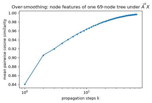
The similarity starts high, because the four-number features of different nodes are already alike, and climbs toward 1: after 16 steps the rows of \hat{\mathbf{A}}^k\mathbf{X} are nearly parallel. Only the degree of a node, through the factor \sqrt{\tilde d_i} of the dominant eigenvector, still differs, and the type of the node has been averaged away. Over-smoothing is a property of the graph and the normalisation, and no weights can undo it entirely.
The train accuracy of the plain 16-layer model equals its test accuracy, and both equal the majority rate: it has not learned the training set. It is an optimisation failure. Signal that has been averaged through many layers with ReLUs and weight decay leaves a gradient that points nowhere useful, and training stays on the plateau where every event is called negative. Residual connections give each node a direct path for its own features and the gradient a direct path through the stack, and the same 16 layers then train and reach 0.948, between the 4- and the 8-layer plain models (0.938 and 0.959). Depth was not the problem. Smoothing without a path for the node’s own features was.
Step 7: a direction-aware layer
The GCN’s symmetric adjacency treats a node’s gate, its siblings and its inputs alike. The property being learned does not: it depends only on the gates above the event. A layer that keeps the two directions apart can express “every gate above me is an OR” directly. The direction-aware layer has three weight matrices:
one for the node itself, one for the message from the node’s gate (its parent; zero for the top
event) and one for the mean of the messages from its inputs (its children; zero for a basic event).
It is two index_add_ calls on the directed edge list. After L layers, information about
the gate L levels above has reached a node through \mathbf{W}_p only, with nothing diluted by
siblings.
class DirGNN(nn.Module):
    def __init__(self, L, hidden=32):
        super().__init__()
        self.inp = nn.Linear(4, hidden)
        self.Ws = nn.ModuleList(nn.Linear(hidden, hidden) for _ in range(L))
        self.Wp = nn.ModuleList(nn.Linear(hidden, hidden, bias=False) for _ in range(L))
        self.Wc = nn.ModuleList(nn.Linear(hidden, hidden, bias=False) for _ in range(L))
        self.out = nn.Linear(hidden, 2)

    def forward(self, g):
        h = self.inp(g.x)
        for Ws, Wp, Wc in zip(self.Ws, self.Wp, self.Wc):
            from_gate = torch.zeros_like(h).index_add_(0, g.child, h[g.par])
            from_inputs = torch.zeros_like(h).index_add_(0, g.par, h[g.child])
            from_inputs = from_inputs / g.n_children[:, None]
            h = torch.relu(Ws(h) + Wp(from_gate) + Wc(from_inputs))
        return self.out(h)


dir_acc = {}
print("direction-aware model")
print("  L   overall   depth1   depth2   depth3   depth4")
for L in (2, 3, 4):
    torch.manual_seed(0)
    dir_model = fit(DirGNN(L), g_train)
    dir_acc[L] = evaluate(dir_model, g_test)
    print(f"{L:3d}   " + "   ".join(f"{a:.3f} " for a in dir_acc[L]))
dir4 = dir_model

depths = [1, 2, 3, 4]
plt.figure(figsize=(7, 4))
for L in (1, 2, 4):
    plt.plot(depths, gcn_acc[L][1:], marker="o", label=f"GCN, L = {L}")
plt.plot(depths, dir_acc[4][1:], marker="s", color="k", label="direction-aware, L = 4")
plt.axhline(majority, color="grey", linestyle=":", label="majority class")
plt.xticks(depths)
plt.xlabel("depth of the basic event below the top event")
plt.ylabel("test accuracy")
plt.title("Accuracy by depth: receptive field and direction")
plt.legend(loc="lower left")
plt.show()
direction-aware model
  L   overall   depth1   depth2   depth3   depth4
  2   0.853    1.000    1.000    0.797    0.843
  3   0.941    1.000    1.000    1.000    0.882
  4   1.000    1.000    1.000    1.000    1.000
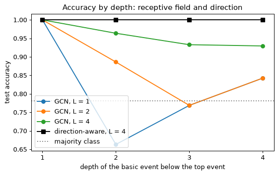
At L = 2 the direction-aware model is better than the GCN of the same depth, and its accuracy is perfect for exactly those events its receptive field reaches: events at depth 1 and 2, whose gates are one and two hops up. At L = 3 it is perfect up to depth 3, and at L = 4 it labels every basic event correctly. This is what an architecture with the right inductive bias does: the network’s capacity is not spent learning that direction matters, and its limits are the ones the receptive field predicts.
Step 8: apply the model to the cooling system
The trained L = 4 direction-aware model has never seen the hand-built tree. Applying it is the last check: it must find E1, E5 and E6, the answer of Step 2. The block also draws the tree, using the layout of Section 8, with the predicted single points of failure marked.
dir4.eval()
with torch.no_grad():
    pred_cool = dir4(g_cool).argmax(1).numpy()
predicted = [NAMES[v] for v in np.where((pred_cool == 1) & (cooling["type"] == BASIC))[0]]
print("single points of failure predicted for the cooling system:", predicted)

pos = {0: (340, 40), 1: (130, 130), 2: (530, 130), 3: (340, 130), 4: (50, 230), 5: (130, 230),
       6: (210, 230), 7: (450, 230), 8: (530, 230), 9: (610, 230), 10: (570, 320),
       11: (650, 320)}
fig, ax = plt.subplots(figsize=(8, 4.2))
for v, p in enumerate(cooling["parent"]):
    if p >= 0:
        ax.plot([pos[v][0], pos[p][0]], [-pos[v][1], -pos[p][1]], color="grey", zorder=1)
for v, (px, py) in pos.items():
    kind = ["OR", "AND", "event"][cooling["type"][v]]
    hit = pred_cool[v] == 1 and cooling["type"][v] == BASIC
    ax.scatter(px, -py, s=900, zorder=2, marker="s" if kind != "event" else "o",
               color="tab:red" if hit else ("white" if kind == "event" else "lightgrey"),
               edgecolor="k")
    ax.text(px, -py, f"{NAMES[v]}\n{kind}" if kind != "event" else NAMES[v],
            ha="center", va="center", fontsize=8, zorder=3)
ax.set_title("Cooling-system fault tree: predicted single points of failure in red")
ax.set_xlabel("layout position (arbitrary units)")
ax.set_ylabel("level (top at the top)")
ax.set_yticks([])
plt.show()
single points of failure predicted for the cooling system: ['E1', 'E5', 'E6']
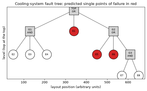
The model names E1, E5 and E6 and nothing else. A small tree being correct is not strong evidence on its own. The test set is the evidence, and this tree is a sanity check that the generator’s trees and the hand-drawn one follow the same rules.
What you should see
- Accuracy by depth shows the receptive field: an L-layer model is reliable only for events at most L hops below the top. The direction-aware model makes this exact: accuracy 1.0 at every depth up to L.
- The undirected GCN improves up to about 4 layers (0.938) and peaks at 8 (0.959). The plain 12- and 16-layer models then predict the majority class for every event. Their node features are nearly identical (the untrained \hat{\mathbf{A}}^k\mathbf{X} similarity climbs toward 1), and with no residual path a deep stack also trains poorly. Residual connections restore it.
- A symmetric adjacency gives each event a mixture of its gate, its siblings and, two hops away, their gate’s other inputs. The property depends only on the gates above. Separate parent and child weights let the network compute “every gate above is OR” exactly.
- The rule that sounds right (“its gate is OR”) is worse than the majority class. Every model must be compared with both.
Try this
- Split by node. Instead of splitting by tree, take a random 70/30 split over all nodes of all 300 trees (all nodes visible in one graph, only the labels hidden) and compare the accuracies. Explain why a per-node split flatters a model that will be used on new trees.
- A depth feature. Add each node’s depth as a fifth feature and retrain the undirected GCN with L = 4. Does it close the gap to the direction-aware model? What does the answer say about what the symmetric layers were missing?
- Predict which nodes are basic events. Train a 2-layer GCN to predict whether a node is a basic event, and compare it with the baseline you named in Exercise 9. What has the GCN learned? This one is best tried after the exercise.
Lab 4 — A physics-informed network for a damped oscillator: forward, failure, fixes and an inverse problem
Goal. You build the physics-informed network of Section 9 for a problem whose exact answer is known, the damped oscillator
with \omega_0 = 2\pi rad/s and \zeta = 0.1, on t \in [0, 2] s. Because the exact solution is known you can measure the error, which is what makes the failures visible. You first train the network the obvious way and watch it converge to the trivial solution u = 0, which satisfies the equation exactly and the initial conditions not at all. You then repair it two ways: by changing the loss weights and by changing the units (a third repair, building the initial condition into the network, is an extension). Last you treat \zeta as unknown, recover it from twelve noisy readings, and compare the result with a classical least-squares fit of the closed form. The data are generated in the lab, nothing is downloaded, and the lab runs in about three minutes on a laptop CPU (190 s in the run shown). You need NumPy, SciPy, PyTorch and matplotlib. Printed numbers may differ from yours in the last digits.
Step 1: the problem and its exact solution
For \zeta < 1 the solution with these initial conditions is
You can check it against the two conditions: at t = 0 it gives 1, and its derivative at 0 is -\zeta\omega_0 + \zeta\omega_0 = 0. The code also fixes the working conventions. The thread count is set to one: a network this small does too little arithmetic per step to gain from several threads, and a single thread avoids the large slowdowns that appear when other programs compete for the cores (in a prototype a step took about 1.2 ms either way when the machine was idle, and about 30 ms with four threads when it was busy). The error measure is the relative L2 error on 1,000 test times, \lVert u_\theta - u\rVert_2 / \lVert u\rVert_2, which is 1 for a network that outputs zero.
import time

import matplotlib.pyplot as plt
import numpy as np
import torch
import torch.nn as nn
from scipy.optimize import curve_fit

torch.manual_seed(0)
torch.set_num_threads(1)

ZETA, W0, T_END = 0.1, 2 * np.pi, 2.0


def exact(t, zeta=ZETA):
    """Closed-form solution of u'' + 2 zeta w0 u' + w0^2 u = 0, u(0) = 1, u'(0) = 0."""
    wd = W0 * np.sqrt(1.0 - zeta**2)
    return np.exp(-zeta * W0 * t) * (np.cos(wd * t) + (zeta * W0 / wd) * np.sin(wd * t))


def rel_l2(u_pred, u_true):
    return float(np.linalg.norm(u_pred - u_true) / np.linalg.norm(u_true))


t_test = np.linspace(0.0, T_END, 1000)
u_test = exact(t_test)
print(f"damped frequency {W0 * np.sqrt(1 - ZETA**2) / (2 * np.pi):.4f} Hz")
print(f"u(0) = {exact(0.0):.4f}, u(0.25 s) = {exact(0.25):.4f}, u(2 s) = {exact(2.0):.4f}")
print(f"largest |u| after 1 s: {np.abs(u_test[t_test > 1.0]).max():.4f}")

plt.figure(figsize=(7, 3.2))
plt.plot(t_test, u_test, color="black")
plt.xlabel("time t (s)")
plt.ylabel("displacement u")
plt.title("Exact solution: damped oscillator, w0 = 2 pi rad/s, zeta = 0.1")
plt.show()
damped frequency 0.9950 Hz
u(0) = 1.0000, u(0.25 s) = 0.0926, u(2 s) = 0.2822
largest |u| after 1 s: 0.5318
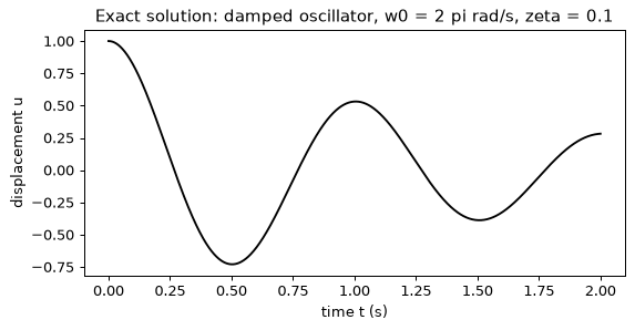
The oscillator completes two periods in the interval and its envelope falls to about 29% of the initial amplitude. Remember these two facts: a network must reproduce two oscillations, and the amplitude it is asked to reproduce is of order 1.
Step 2: the network, its derivatives and the loss
The network u_\theta(t) is a multilayer perceptron with three hidden layers of 32 tanh units. It divides its input by the interval length, so that the first layer sees numbers in [0, 1] whatever the units. The smooth tanh matters: the residual needs two derivatives of the network, and a ReLU network has a second derivative that is zero almost everywhere.
The derivative helper is the whole mechanism of a PINN. torch.autograd.grad differentiates the
output with respect to the input time, and create_graph=True keeps the derivative itself
differentiable, so that it can be differentiated again (for u'') and so that the loss built from
it can be differentiated with respect to the weights. The residual of the equation is written
for any coefficients c_1, c_2, as u'' + c_1 u' + c_2 u; the dimensional problem has
c_1 = 2\zeta\omega_0 and c_2 = \omega_0^2, and Step 6 will use another pair. The loss of
Section 9 is
with N = 200 evenly spaced collocation points. The fit function trains for a given number of
steps with Adam at learning rate 10^{-3}, and records the two loss terms, the test error and the
largest |u_\theta| on the test times at the steps you ask for.
class PINN(nn.Module):
    def __init__(self, t_scale, width=32):
        super().__init__()
        self.t_scale = t_scale  # input is divided by the interval length
        self.net = nn.Sequential(
            nn.Linear(1, width), nn.Tanh(),
            nn.Linear(width, width), nn.Tanh(),
            nn.Linear(width, width), nn.Tanh(),
            nn.Linear(width, 1),
        )

    def forward(self, t):
        return self.net(t / self.t_scale)


def d(u, t):
    """du/dt by autograd; create_graph keeps the result differentiable."""
    return torch.autograd.grad(u, t, torch.ones_like(u), create_graph=True)[0]


def loss_terms(model, t_col, t_zero, c1, c2):
    u = model(t_col)
    u_t = d(u, t_col)
    u_tt = d(u_t, t_col)
    residual = (u_tt + c1 * u_t + c2 * u).pow(2).mean()
    u0 = model(t_zero)
    initial = (u0 - 1.0).pow(2).mean() + d(u0, t_zero).pow(2).mean()
    return residual, initial


def fit(t_end, c1, c2, lam_ic, steps, log_at=(), lr=1e-3, seed=0):
    """Train a PINN; return the model and a log of (step, residual, ic, error, max|u|)."""
    torch.manual_seed(seed)
    model = PINN(t_end)
    opt = torch.optim.Adam(model.parameters(), lr=lr)
    t_col = torch.linspace(0.0, t_end, 200).reshape(-1, 1).requires_grad_(True)
    t_zero = torch.zeros(1, 1, requires_grad=True)
    t_eval = torch.tensor(t_test / T_END * t_end, dtype=torch.float32).reshape(-1, 1)
    log, curve = [], []
    t0 = time.time()
    for step in range(steps + 1):
        residual, initial = loss_terms(model, t_col, t_zero, c1, c2)
        if step % 100 == 0 or step in log_at:
            with torch.no_grad():
                u_hat = model(t_eval).numpy().ravel()
            err = rel_l2(u_hat, u_test)
            curve.append((step, err))
            if step in log_at:
                log.append((step, residual.item(), initial.item(), err, np.abs(u_hat).max()))
        if step == steps:
            break
        loss = residual + lam_ic * initial
        opt.zero_grad()
        loss.backward()
        opt.step()
    ms = 1000 * (time.time() - t0) / steps
    return model, log, curve, ms


def show(log):
    print("  step   residual   ic term   rel. L2 error   max|u|")
    for step, res, ic, err, umax in log:
        print(f"{step:6d}   {res:8.2e}   {ic:7.4f}   {err:13.4f}   {umax:6.4f}")


# one forward pass at initialisation: the sizes of the two loss terms
model0 = PINN(T_END)
t_col0 = torch.linspace(0.0, T_END, 200).reshape(-1, 1).requires_grad_(True)
t_zero0 = torch.zeros(1, 1, requires_grad=True)
res0, ic0 = loss_terms(model0, t_col0, t_zero0, 2 * ZETA * W0, W0**2)
print(f"at initialisation: residual {res0.item():.2f}, initial conditions {ic0.item():.2f}")
print(f"parameters: {sum(p.numel() for p in model0.parameters())}")
at initialisation: residual 52.46, initial conditions 1.36
parameters: 2209
The residual term is already about forty times larger than the initial-condition term before any training. That is not an accident of the initialisation. The equation contains \omega_0^2 \approx 39.5, so a unit error in u costs a residual of order 40 and a squared residual of order 1,500, while the same unit error in u(0) costs 1. The two terms live on scales that differ by three orders of magnitude, and the optimiser follows the larger one.
Step 3: the obvious loss, and the trivial solution
Now train in the problem’s own units, with the two terms weighted equally (\lambda_{\text{ic}} = 1), for 3,000 steps. Use the dimensional coefficients and the interval [0, 2].
C1_DIM, C2_DIM = 2 * ZETA * W0, W0**2
model_a, log_a, curve_a, ms = fit(T_END, C1_DIM, C2_DIM, 1.0, 3000, log_at=(0, 1000, 3000))
show(log_a)
print(f"{ms:.1f} ms per step")

with torch.no_grad():
    u_a = model_a(torch.tensor(t_test, dtype=torch.float32).reshape(-1, 1)).numpy().ravel()
plt.figure(figsize=(7, 3.2))
plt.plot(t_test, u_test, color="black", label="exact")
plt.plot(t_test, u_a, color="tab:red", label="PINN, lambda_ic = 1")
plt.xlabel("time t (s)")
plt.ylabel("displacement u")
plt.title("Dimensional units, equal weights: the trivial solution")
plt.legend()
plt.show()
  step   residual   ic term   rel. L2 error   max|u|
     0   5.25e+01    1.3626          1.0914   0.1951
  1000   3.14e-03    0.9922          0.9993   0.0039
  3000   5.92e-03    0.9877          0.9986   0.0063
5.1 ms per step
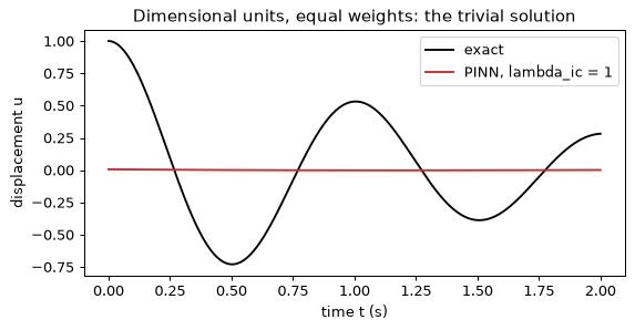
The loss has fallen to a small number and the answer is wrong. The residual term is tiny, the initial-condition term has barely moved from its starting value of about 1, and the network outputs a curve of size 0.01 that has nothing to do with the oscillation. The relative error is close to 1. This is the failure mode of Section 9 in its cleanest form: u \equiv 0 is a solution of the differential equation, so the residual can be driven to zero by switching the network off, and the initial conditions, which are the only thing that distinguishes the wanted solution from zero, have a gradient too weak to resist. Nothing in the printed loss warns you. Only a comparison with a known answer (or with measurements) does.
Step 4: remove the initial conditions altogether
To confirm that the conditions are the only barrier, set \lambda_{\text{ic}} = 0. Now nothing at all distinguishes the wanted solution from zero.
model_b, log_b, curve_b, _ = fit(T_END, C1_DIM, C2_DIM, 0.0, 3000, log_at=(0, 3000))
show(log_b)
  step   residual   ic term   rel. L2 error   max|u|
     0   5.25e+01    1.3626          1.0914   0.1951
  3000   5.07e-06    1.0002          1.0000   0.0001
The residual falls to about 5\times10^{-6}, three orders of magnitude below that of the previous run, and the network’s amplitude is of order 10^{-4}. The error is 1.000: the network has found exactly the function with zero residual that is easiest to find. A well-posed problem needs its conditions, and a loss that does not make the conditions binding has a trivial minimum.
Step 5: the first fix, a large weight on the conditions
Raise \lambda_{\text{ic}} to 100, so that the two terms are of comparable size when the network is wrong in the way that matters, and train for 10,000 steps. Training is longer because the problem is harder than it looks: two periods of a decaying oscillation are being fitted by a function that starts out almost flat.
model_c, log_c, curve_c, _ = fit(
    T_END, C1_DIM, C2_DIM, 100.0, 10000, log_at=(0, 1000, 5000, 10000)
)
show(log_c)
  step   residual   ic term   rel. L2 error   max|u|
     0   5.25e+01    1.3626          1.0914   0.1951
  1000   5.24e+00    0.0086          0.3306   0.9071
  5000   1.07e-01    0.0000          0.0152   0.9973
 10000   1.89e-02    0.0000          0.0039   0.9992
The weight works, and slowly: the error is still 33% after 1,000 steps, about 1.5% after 5,000 and 0.4% after 10,000. The residual term, which stays far above zero for thousands of steps, shows how hard the optimiser is pulled between the two terms. The cost is a hyperparameter. A weight of 100 was chosen here because we could see the failure at weight 1; with an unknown solution there is no error to look at, and the weight has to be found by trial or by an adaptive scheme (see Section 9).
Step 6: the second fix, non-dimensionalise
The deeper cause is the units. Define the dimensionless time \hat t = \omega_0 t, which runs over [0, 4\pi] for our interval. The chain rule gives \mathrm{d}/\mathrm{d}t = \omega_0\, \mathrm{d}/\mathrm{d}\hat t, so
with the same initial conditions, u(0) = 1 and u_{\hat t}(0) = 0. The coefficients are now c_1 = 2\zeta = 0.2 and c_2 = 1, all terms are of order 1, and the residual and the initial-condition term are comparable without any hand-tuned weight. The network is the same, the weight is back to 1, and only the coordinate has changed.
C1_ND, C2_ND = 2 * ZETA, 1.0
model_d, log_d, curve_d, ms = fit(
    4 * np.pi, C1_ND, C2_ND, 1.0, 10000, log_at=(0, 2500, 5000, 7500, 10000)
)
show(log_d)
print(f"{ms:.1f} ms per step")
  step   residual   ic term   rel. L2 error   max|u|
     0   3.37e-02    1.3623          1.0914   0.1951
  2500   4.67e-03    0.0000          0.3892   0.9946
  5000   2.84e-04    0.0000          0.0603   1.0004
  7500   4.35e-07    0.0000          0.0004   1.0002
 10000   9.52e-06    0.0000          0.0073   1.0039
4.8 ms per step
The initial residual is now 0.034 rather than 52, so the imbalance of Step 2 has gone, and
indeed reversed: the initial-condition term (1.36) is now the larger one, and the optimiser
satisfies it first and then fits the oscillation. Training is not faster at the start (the error
is 0.39 after 2,500 steps and 0.06 after 5,000, against 0.015 at 5,000 for the weighted run),
but it keeps improving, reaches 0.0004 at 7,500 steps, ten times below the weighted run’s final
0.0039, and does so with no tuned weight. It does not stay there. At step 10,000 the printed error
is 0.0073, because Adam at a fixed learning rate of 10^{-3} keeps kicking the network away from
the minimum: in a copy of this lab that printed curve_d, the error recorded every 100 steps
jumps between about 0.0001 and 0.016 after step 6,000, and is lowest (0.00006) at step 8,700.
The weighted run oscillates too, between 0.004 and 0.013 over its last 1,000 steps. A decaying
learning rate, or keeping the best checkpoint by a validation measure, is the usual remedy; the
point here is that the non-dimensional form reaches the low error without a weight. (The
residuals of the two runs cannot be compared directly, because the equations differ by the
factor \omega_0^2.) The lesson is general and transfers beyond this equation:
before reaching for loss-balancing schemes, put the equation in a form where its terms are of
order 1.
The convergence curves recorded during the three runs show it directly.
fig, ax = plt.subplots(1, 2, figsize=(10, 3.6))
for curve, label, colour in [
    (curve_a, "dimensional, weight 1", "tab:red"),
    (curve_c, "dimensional, weight 100", "tab:orange"),
    (curve_d, "non-dimensional, weight 1", "tab:blue"),
]:
    steps_, errs = zip(*curve)
    ax[0].semilogy(steps_, errs, label=label, color=colour)
ax[0].set_xlabel("training step")
ax[0].set_ylabel("relative L2 error")
ax[0].set_title("Error against the exact solution")
ax[0].legend()

with torch.no_grad():
    u_d = model_d(torch.tensor(W0 * t_test, dtype=torch.float32).reshape(-1, 1))
ax[1].plot(t_test, u_test, color="black", label="exact")
ax[1].plot(t_test, u_d.numpy().ravel(), "--", color="tab:blue", label="PINN, non-dimensional")
ax[1].set_xlabel("time t (s)")
ax[1].set_ylabel("displacement u")
ax[1].set_title("The repaired network")
ax[1].legend()
plt.tight_layout()
plt.show()
Step 7: the inverse problem
Now the damping ratio is unknown. Twelve displacement readings are generated at random times in [0, 2] s from the exact solution with \zeta = 0.1 and Gaussian noise of standard deviation 0.02, as twelve accelerometer-derived samples might be. The network is non-dimensional as in Step 6. The unknown enters the residual as a trainable scalar, parameterised as \log\zeta so that it stays positive, starting from \zeta = 0.5, a value five times too large. The loss adds a data term, ten times the mean squared error at the readings; the weight 10 states that the readings are trusted a little more than the physics is satisfied at a single collocation point. Network weights and \log\zeta are optimised together by the same Adam.
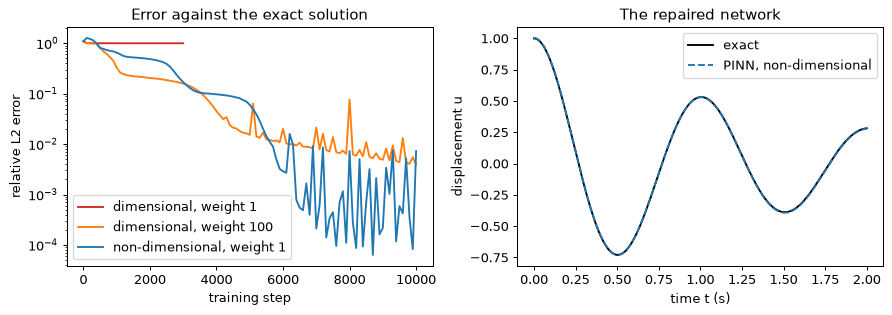
g = torch.Generator().manual_seed(1)
t_meas = T_END * torch.rand(12, generator=g)
y_meas = torch.tensor(exact(t_meas.numpy()), dtype=torch.float32) + 0.02 * torch.randn(
    12, generator=g
)
th_meas = (W0 * t_meas).reshape(-1, 1)  # readings in the non-dimensional time


def fit_inverse(steps=10000, lr=1e-3, seed=0, w_data=10.0):
    torch.manual_seed(seed)
    model = PINN(4 * np.pi)
    log_zeta = nn.Parameter(torch.log(torch.tensor(0.5)))
    opt = torch.optim.Adam(list(model.parameters()) + [log_zeta], lr=lr)
    t_col = torch.linspace(0.0, 4 * np.pi, 200).reshape(-1, 1).requires_grad_(True)
    t_zero = torch.zeros(1, 1, requires_grad=True)
    t_eval = torch.tensor(W0 * t_test, dtype=torch.float32).reshape(-1, 1)
    path = []
    for step in range(steps + 1):
        zeta = log_zeta.exp()
        residual, initial = loss_terms(model, t_col, t_zero, 2 * zeta, 1.0)
        data = (model(th_meas).squeeze(1) - y_meas).pow(2).mean()
        if step % 1000 == 0:
            with torch.no_grad():
                err = rel_l2(model(t_eval).numpy().ravel(), u_test)
            path.append((step, zeta.item(), err))
        if step == steps:
            break
        loss = residual + initial + w_data * data
        opt.zero_grad()
        loss.backward()
        opt.step()
    return model, zeta.item(), path


model_e, zeta_hat, path = fit_inverse()
print("  step   zeta    solution error")
for step, z, err in path:
    print(f"{step:6d}   {z:.4f}   {err:.4f}")
print(f"recovered zeta = {zeta_hat:.4f} (true {ZETA})")
  step   zeta    solution error
     0   0.5000   1.0914
  1000   0.4235   0.2269
  2000   0.2372   0.1180
  3000   0.1736   0.0806
  4000   0.1400   0.0599
  5000   0.1201   0.0473
  6000   0.1087   0.0345
  7000   0.1030   0.0305
  8000   0.1007   0.0169
  9000   0.0996   0.0181
 10000   0.0987   0.0192
recovered zeta = 0.0987 (true 0.1)
Starting five times too high, the estimate falls to 0.12 by step 5,000 and settles at 0.0987, 1.3% below the true 0.1. The solution error ends at about 0.019. Noise of 0.02 on a signal whose root-mean-square value is 0.44 is a relative error of about 0.046 at the twelve readings, so the network’s solution is closer to the truth than the readings are: the equation filters the noise. Twelve readings and an equation are enough because the equation supplies the shape of the curve and the readings only have to pin down one number. The solution error is not as small as Step 6’s best (0.0004) because the data term pulls the network toward noisy points.
Step 8: the classical baseline
The honest comparison for a one-parameter inverse problem with a closed form is a least-squares
fit of the closed form to the same readings. curve_fit minimises the squared difference between
exact(t, zeta) and the readings, and returns an uncertainty from the curvature of the fit.
popt, pcov = curve_fit(
    lambda t, z: exact(t, z), t_meas.numpy(), y_meas.numpy(), p0=[0.5], bounds=(0.01, 0.99)
)
print(f"curve_fit: zeta = {popt[0]:.4f} +/- {np.sqrt(pcov[0, 0]):.4f}")
print(f"PINN:      zeta = {zeta_hat:.4f}")

fig, ax = plt.subplots(1, 2, figsize=(10, 3.6))
ax[0].plot(t_test, u_test, color="black", label="exact (zeta = 0.1)")
with torch.no_grad():
    u_e = model_e(torch.tensor(W0 * t_test, dtype=torch.float32).reshape(-1, 1)).numpy()
ax[0].plot(t_test, u_e.ravel(), "--", color="tab:blue", label="PINN, inverse problem")
ax[0].scatter(t_meas.numpy(), y_meas.numpy(), color="tab:red", zorder=3, label="12 readings")
ax[0].set_xlabel("time t (s)")
ax[0].set_ylabel("displacement u")
ax[0].set_title("Twelve noisy readings and the recovered solution")
ax[0].legend()
steps_p, zetas, _ = zip(*path)
ax[1].plot(steps_p, zetas, "o-", color="tab:blue", label="PINN estimate")
ax[1].axhline(ZETA, color="black", label="true value")
ax[1].axhline(popt[0], color="tab:green", linestyle="--", label="curve_fit")
ax[1].set_xlabel("training step")
ax[1].set_ylabel("damping ratio zeta")
ax[1].set_title("The estimate of zeta during training")
ax[1].legend()
plt.tight_layout()
plt.show()
curve_fit: zeta = 0.0977 +/- 0.0015
PINN:      zeta = 0.0987
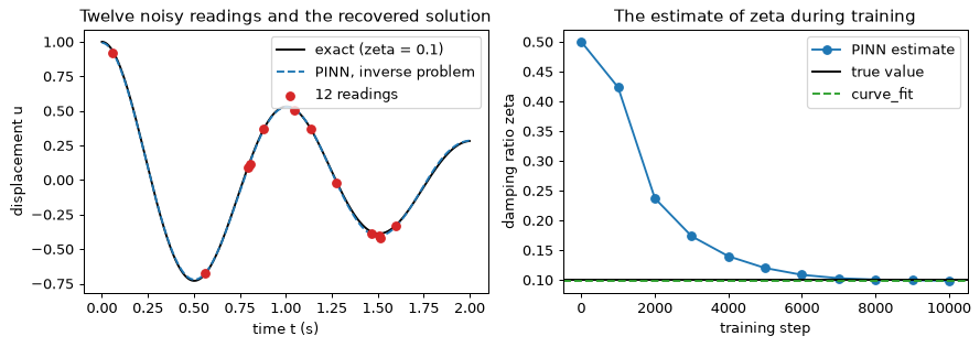
The two estimates, 0.0977 and 0.0987, differ by about two thirds of the fit’s own standard error of 0.0015, and the true value 0.1 is about 1.5 standard errors from the least-squares one: both are consistent with the truth and with each other. This is the correct conclusion, not a disappointing one. When the solution is a closed form with one unknown, a least-squares fit is faster, returns an error bar, and cannot get stuck in a trivial solution. The PINN earns its cost when no closed form exists: a nonlinear equation, an irregular geometry, an unknown that is a spatial field. The lab’s value is that you have seen every step on a problem small enough to check.
What you should see
- In dimensional units the residual term starts about 40 times larger than the initial-condition term (52.5 against 1.4). With equal weights the optimiser drives the network to nearly zero: the loss is small (residual 0.006) and the relative error is 0.999. Without initial conditions the result is the same, with a residual of 5\times10^{-6}. The trivial solution satisfies the equation exactly.
- Weighting the initial conditions by 100 fixes it (error 0.0039 after 10,000 steps); non-dimensionalising fixes it with no weight, because the terms of the equation are all of order 1, and reaches lower errors (0.0004 at 7,500 steps), though at a fixed learning rate the error jumps about and reads 0.0073 at 10,000.
- The inverse problem recovers \zeta = 0.0987 from twelve noisy readings, within 1.3% of the true value and consistent with the least-squares fit of the closed form (0.0977 \pm 0.0015). When a closed form exists, use it; the PINN earns its cost when it does not.
- Second derivatives through autograd cost several forward and backward passes, yet this network takes about 5 ms per step, so the whole lab runs in about three minutes on a CPU. The cost is in the number of steps (7,500 to reach 0.0004), not in the step.
Try this
- Hard constraint. Build the initial conditions into the network, u_\theta(t) = 1 + (t/t_{\text{end}})^2\,N_\theta(t), which equals 1 at t = 0 and has zero derivative there whatever N_\theta is. Drop the initial-condition term, and train in dimensional units for 10,000 steps. A trivial solution is no longer possible, so the failure of Step 3 cannot occur. Is the error nonetheless still large, and why? (The scaling problem has not gone away.)
- Spectral bias. Set \omega_0 = 8\pi (eight periods in the 2 s) and train the non-dimensional form again; the network now needs eight oscillations. Then add Fourier features [\sin k\hat t, \cos k\hat t] for k = 1, 2, 4 as extra inputs and compare the two runs. Why does a tanh network with inputs of size 1 struggle with high frequencies?
- From ODE to PDE. Exercise e12 starts from this code and moves to the heat equation, where the collocation points become a grid in space and time.
Lab 5 — Contrastive pretraining on unlabelled vibration signals
Goal. You pretrain an encoder with the InfoNCE loss of Section 11 on machine-vibration windows whose labels are never shown to it, and measure what that bought with a linear probe: a logistic regression trained on only 5, 20 or 100 labelled windows per class. The comparison is against the two things an engineer would try first, the raw waveform and its spectral magnitudes, and against an encoder that was never trained. Then you remove the augmentations one at a time and watch the representation get worse, which is the point of the lab: in contrastive learning the augmentations are the supervision. The vibration data are generated in the lab (four classes, random phases), so nothing is downloaded, and the lab runs in one to two minutes on a laptop CPU. You need NumPy, scikit-learn, PyTorch and matplotlib. Printed numbers may differ from yours in the last digits.
Step 1: a generator of vibration windows
A real rotating machine would be recorded with an accelerometer. Here a window is one second at 256 Hz, so 256 samples, of a shaft turning at a speed f_r drawn uniformly from 9 to 11 Hz. The four classes differ in the harmonics of f_r they contain:
| class | signal (before noise) |
|---|---|
| 0 healthy | 1.0\sin(2\pi f_r t + \varphi_1) + 0.2\sin(2\pi\,2 f_r t + \varphi_2) |
| 1 imbalance | the same with the 1x amplitude raised to 2.5 |
| 2 misalignment | 1x, 2x and 3x components with amplitudes 1.0, 1.5 and 0.5 |
| 3 bearing defect | healthy, plus impulses repeating at 3.57 f_r, each a 60 Hz oscillation of amplitude 1.5 decaying as e^{-30\tau} |
All phases are random, the sensor gain is uniform on 0.8 to 1.2, and Gaussian noise of standard deviation 0.3 is added. The random phases are the heart of the problem. They are what a real recording looks like when the window starts at an arbitrary moment of the cycle, and they mean that two windows of the same class share no sample values. The label depends on the amplitudes of the harmonics, not on the phases.
The impulse train is built from the time \tau since the last impulse, which is (t - t_0) modulo the impulse period 1/(3.57 f_r); this gives the full decaying oscillation after each impulse in one vectorised line.
import time

import matplotlib.pyplot as plt
import numpy as np
import torch
import torch.nn as nn
import torch.nn.functional as F
from sklearn.linear_model import LogisticRegression
from sklearn.metrics import confusion_matrix
from sklearn.preprocessing import StandardScaler

np.random.seed(0)
torch.manual_seed(0)
rng = np.random.default_rng(0)

FS, N_SAMPLES = 256, 256
T = np.arange(N_SAMPLES) / FS
CLASS_NAMES = ["healthy", "imbalance", "misalignment", "bearing defect"]


def make_windows(n, rng):
    labels = rng.integers(0, 4, size=n)
    f_r = rng.uniform(9.0, 11.0, size=(n, 1))
    ph = rng.uniform(0.0, 2 * np.pi, size=(n, 3))

    def wave(k, i):  # k-th harmonic of the shaft speed with its own random phase
        return np.sin(2 * np.pi * k * f_r * T + ph[:, i:i + 1])

    amp = np.array([[1.0, 0.2, 0.0],      # healthy: amplitudes of 1x, 2x, 3x
                    [2.5, 0.2, 0.0],      # imbalance
                    [1.0, 1.5, 0.5],      # misalignment
                    [1.0, 0.2, 0.0]])[labels]  # bearing defect: healthy + impulses
    x = amp[:, 0:1] * wave(1, 0) + amp[:, 1:2] * wave(2, 1) + amp[:, 2:3] * wave(3, 2)
    period = 1.0 / (3.57 * f_r)
    t0 = rng.uniform(0.0, 1.0, size=(n, 1)) * period
    tau = np.mod(T - t0, period)  # time since the most recent impulse
    impulses = 1.5 * np.exp(-30.0 * tau) * np.sin(2 * np.pi * 60.0 * tau)
    x = x + (labels == 3)[:, None] * impulses
    x = x * rng.uniform(0.8, 1.2, size=(n, 1)) + 0.3 * rng.standard_normal((n, N_SAMPLES))
    return x.astype(np.float32), labels


X_pool, y_pool = make_windows(4000, rng)  # pretraining pool; labels kept aside
X_test, y_test = make_windows(2000, rng)
print(X_pool.shape, X_test.shape)
print("class counts in the pool:", np.bincount(y_pool))
print(f"signal standard deviation {X_pool.std():.3f}")

fig, axes = plt.subplots(2, 4, figsize=(13, 4.8))
spec_axis = np.fft.rfftfreq(N_SAMPLES, 1 / FS)
for c in range(4):
    x = X_pool[np.flatnonzero(y_pool == c)[0]]
    axes[0, c].plot(T, x, color="black", linewidth=0.8)
    axes[0, c].set_title(CLASS_NAMES[c])
    axes[0, c].set_xlabel("time (s)")
    axes[1, c].plot(spec_axis, np.abs(np.fft.rfft(x)) / N_SAMPLES * 2, color="tab:blue")
    axes[1, c].set_xlabel("frequency (Hz)")
    axes[1, c].set_xlim(0, 128)
axes[0, 0].set_ylabel("acceleration (a.u.)")
axes[1, 0].set_ylabel("spectral magnitude")
fig.suptitle("One window of each class (top) and its magnitude spectrum (bottom)")
plt.tight_layout()
plt.show()
(4000, 256) (2000, 256)
class counts in the pool: [ 986  985  991 1038]
signal standard deviation 1.306
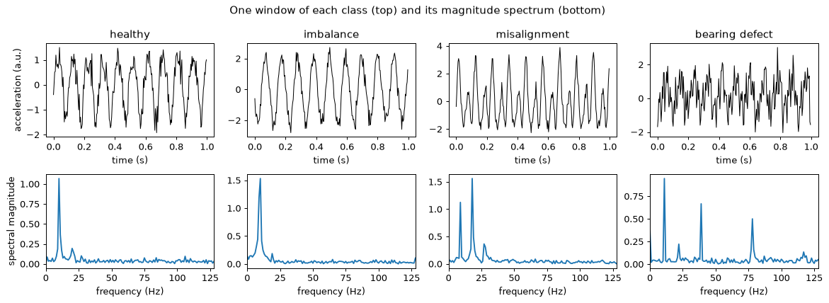
Read the spectra before the waveforms, and note that the vertical axes differ. The healthy window has a peak at about f_r and a small one at 2f_r. The imbalance window has a taller peak at f_r (the 1x amplitude is 2.5 times larger, though the peak height is also reduced by spectral leakage, because the window does not hold a whole number of cycles). The misalignment window has its largest peak at 2f_r and a third at 3f_r. The bearing-defect window adds a comb of peaks at multiples of the impulse rate 3.57 f_r, near 39 and 78 Hz in this window. In the time domain the classes are hard to tell apart by eye, and the phases differ from window to window. The spectra are what an engineer computes by habit, and Step 3 uses them as a baseline.
Step 2: the probe protocol
The quality of a representation is measured by how well a linear classifier does on it with few labels. A linear probe cannot repair a bad representation by learning a clever nonlinear function of it, so its accuracy reflects the features. For each label budget of 5, 20 and 100 windows per class, the helper draws that many labelled windows per class from the pool, five times with different draws, fits a standardised logistic regression on each draw, and averages the accuracy on the 2,000 test windows. The five draws matter at 5 labels per class, where a single draw of 20 windows could be unlucky.
BUDGETS = (5, 20, 100)


def probe(feat_pool, feat_test, budgets=BUDGETS, n_draws=5, seed=0, return_model=False):
    """Mean test accuracy of a logistic regression on a few labelled windows per class."""
    draw_rng = np.random.default_rng(seed)
    accs, last = [], None
    for n_per_class in budgets:
        scores = []
        for _ in range(n_draws):
            idx = np.concatenate([
                draw_rng.choice(np.flatnonzero(y_pool == c), n_per_class, replace=False)
                for c in range(4)
            ])
            scaler = StandardScaler().fit(feat_pool[idx])
            clf = LogisticRegression(max_iter=5000).fit(scaler.transform(feat_pool[idx]),
                                                         y_pool[idx])
            pred = clf.predict(scaler.transform(feat_test))
            scores.append((pred == y_test).mean())
            last = pred
        accs.append(float(np.mean(scores)))
    return (accs, last) if return_model else accs


def fmt(accs):
    return "  ".join(f"{a:.3f}" for a in accs)
Step 3: baselines
Three baselines set the bar. The first is a logistic regression on the 256 raw samples. The second is on the 129 FFT magnitudes: the classical feature for rotating machinery, which discards phase by construction. The third is the encoder of Step 5 before any training, with random weights: a random network is a surprisingly informative featuriser, and any claim that pretraining helps has to beat it.
acc_raw = probe(X_pool, X_test)
fft_pool = np.abs(np.fft.rfft(X_pool, axis=1)).astype(np.float32)
fft_test = np.abs(np.fft.rfft(X_test, axis=1)).astype(np.float32)
acc_fft = probe(fft_pool, fft_test)
print(f"raw waveform (256 features):   {fmt(acc_raw)}")
print(f"FFT magnitude (129 features):  {fmt(acc_fft)}")


class Encoder(nn.Module):
    """h = f(x) is the representation kept after pretraining; z = g(h) feeds the loss."""

    def __init__(self, d_in=256, d_hidden=256, d_h=128, d_z=64):
        super().__init__()
        self.f = nn.Sequential(nn.Linear(d_in, d_hidden), nn.ReLU(), nn.Linear(d_hidden, d_h))
        self.g = nn.Sequential(nn.ReLU(), nn.Linear(d_h, d_z))  # projection head

    def forward(self, x):
        h = self.f(x)
        return h, F.normalize(self.g(h), dim=1)


def embed(model, X):
    with torch.no_grad():
        h, z = model(torch.from_numpy(X))
    return h.numpy(), z.numpy()


torch.manual_seed(0)
untrained = Encoder()
h_pool0, _ = embed(untrained, X_pool)
h_test0, _ = embed(untrained, X_test)
acc_untrained = probe(h_pool0, h_test0)
print(f"untrained encoder, h (128):    {fmt(acc_untrained)}")
raw waveform (256 features):   0.371  0.448  0.473
FFT magnitude (129 features):  0.850  0.899  0.974
untrained encoder, h (128):    0.532  0.738  0.895
Three facts are visible. The raw waveform is far below the others: with random phases no fixed linear combination of the 256 samples identifies a class, which is the problem stated above. The FFT magnitudes are far better, because the magnitude does not depend on the phase, but with five labels per class they reach only about 0.85, and the gap to the best representation of Step 6 is largest there. And the untrained network is already better than the raw waveform, because random nonlinear features of a signal are partly phase-insensitive; it is still far below the FFT at 5 labels per class (0.53 against 0.85), and it is the bar the trained encoder must clear.
Step 4: the loss
The loss is the NT-Xent form of InfoNCE (Section 11). A batch of B windows gives 2B views, two augmentations of each window. Let \mathbf{z}_1, \dots, \mathbf{z}_{2B} be their L2-normalised embeddings, so that the dot product is the cosine similarity. For view i with twin view j(i) the loss is
which is a cross-entropy over the other 2B - 1 views with the twin as the correct class. In code
this is one matrix product, a diagonal set to -\infty (a view is never its own candidate), and
F.cross_entropy with the twin’s index as the target. The temperature \tau divides the
similarities: a small \tau makes the softmax sharp and punishes the hardest negatives.
The sanity check reuses the worked example of Section 11: one anchor with similarities (0.9, 0.2, 0.1, -0.3) to the positive and three negatives. At \tau = 1 the softmax is nearly flat and the loss is 0.81; at \tau = 0.1 the positive dominates and the loss is 0.0013.
def nt_xent(z1, z2, tau):
    """InfoNCE over 2B views; z1[i] and z2[i] are two views of window i (unit vectors)."""
    b = z1.shape[0]
    z = torch.cat([z1, z2], dim=0)                     # 2B x d
    logits = z @ z.T / tau                             # 2B x 2B cosine similarities / tau
    logits.fill_diagonal_(float("-inf"))               # a view is not its own negative
    target = torch.cat([torch.arange(b, 2 * b), torch.arange(0, b)])  # index of the twin
    return F.cross_entropy(logits, target)


sims = torch.tensor([[0.9, 0.2, 0.1, -0.3]])
for tau in (1.0, 0.1):
    print(f"tau = {tau}: loss {F.cross_entropy(sims / tau, torch.tensor([0])).item():.4f}")

# Collapse check: identical embeddings for every view give log(2B - 1).
B = 256
collapsed = F.normalize(torch.ones(B, 64), dim=1)
print(f"collapsed embeddings: {nt_xent(collapsed, collapsed, 0.2).item():.4f}")
print(f"log(2B - 1) = log({2 * B - 1}) = {np.log(2 * B - 1):.4f}")
tau = 1.0: loss 0.8096
tau = 0.1: loss 0.0013
collapsed embeddings: 6.2364
log(2B - 1) = log(511) = 6.2364
The collapse value is the loss of a representation that carries no information: every candidate looks the same, so the softmax is uniform over 2B - 1 = 511 views and the loss is \log 511. Training must bring the loss well below this number, and a loss that sits near it means the encoder has collapsed or the augmentations are too destructive.
Step 5: the augmentations and the pretraining loop
Each view is made by three random operations, chosen to say what must not matter to the
representation: a circular time shift by a random number of samples (the window start is
arbitrary, so the phase must not matter), a gain drawn log-uniformly from 0.8 to 1.25 (the
sensor sensitivity must not matter) and extra noise of standard deviation 0.1. The shift is
done with torch.gather so that every window in the batch gets its own shift. A circular shift
keeps the magnitudes of the spectrum almost exactly and changes the phases, which is the
invariance we want to teach (the wrap-around joins the end of the window to its start, a small
artefact that a real pipeline would avoid by cutting windows from a longer recording).
The encoder is the one built in Step 3. The training uses batches of B = 256 (so each view has its twin and 2B - 2 = 510 views of other windows as negatives), Adam at learning rate 10^{-3}, \tau = 0.2, and 60 epochs over the 4,000 pool windows: 15 batches an epoch, 900 steps. The labels are not used.
def augment(x, gen, shift=True, gain=True, noise=True):
    b, n = x.shape
    if shift:
        s = torch.randint(0, n, (b, 1), generator=gen)
        idx = (torch.arange(n).unsqueeze(0) + s) % n
        x = torch.gather(x, 1, idx)
    if gain:
        x = x * torch.exp(torch.empty(b, 1).uniform_(np.log(0.8), np.log(1.25), generator=gen))
    if noise:
        x = x + 0.1 * torch.randn(x.shape, generator=gen)
    return x


def pretrain(seed=0, epochs=60, batch=256, tau=0.2, lr=1e-3, **aug):
    torch.manual_seed(seed)
    gen = torch.Generator().manual_seed(seed)
    model = Encoder()
    opt = torch.optim.Adam(model.parameters(), lr=lr)
    data = torch.from_numpy(X_pool)
    losses = []
    for epoch in range(epochs):
        order = torch.randperm(len(data), generator=gen)
        for start in range(0, len(data) - batch + 1, batch):  # drop the last short batch
            xb = data[order[start:start + batch]]
            _, z1 = model(augment(xb, gen, **aug))
            _, z2 = model(augment(xb, gen, **aug))
            loss = nt_xent(z1, z2, tau)
            opt.zero_grad()
            loss.backward()
            opt.step()
            losses.append(loss.item())
    return model, losses


t0 = time.time()
model_full, losses_full = pretrain(seed=0)
print(f"{len(losses_full)} steps in {time.time() - t0:.1f} s")
print(f"loss at step 0: {losses_full[0]:.3f}, final loss (mean of last 15): "
      f"{np.mean(losses_full[-15:]):.3f}")
print(f"loss of collapsed embeddings: log(2B - 1) = {np.log(511):.3f}")

plt.figure(figsize=(7, 3.2))
plt.plot(losses_full, color="tab:blue")
plt.axhline(np.log(511), color="grey", linestyle="--", label="log(2B - 1), collapsed")
plt.xlabel("training step")
plt.ylabel("InfoNCE loss")
plt.title("Contrastive pretraining loss (tau = 0.2, B = 256)")
plt.legend()
plt.show()
900 steps in 12.4 s
loss at step 0: 6.150, final loss (mean of last 15): 2.376
loss of collapsed embeddings: log(2B - 1) = 6.236
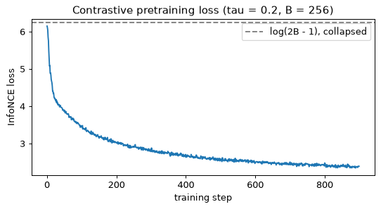
The loss starts at 6.15, close to the collapse value of 6.24, and falls to about 2.4, which is 38% of it. It does not reach zero, and it should not: two views of one window can never be perfectly matched among 510 others while the noise and gain differ, and tending to zero would suggest that the task is trivial.
Step 6: the linear probe on the pretrained representation
The encoder is now used as a frozen feature extractor. The probe is trained on the same labelled draws as the baselines, with the same protocol. Two representations are probed: \mathbf{h}, the 128-dimensional output of the encoder proper, and \mathbf{z}, the 64-dimensional output after the projection head that the loss saw. Two more pretraining runs with other seeds give a feel for the variation.
h_pool, z_pool = embed(model_full, X_pool)
h_test, z_test = embed(model_full, X_test)
acc_h = probe(h_pool, h_test)
acc_z = probe(z_pool, z_test)
print("labels per class:           ", "   ".join(f"{b:>3d}  " for b in BUDGETS))
print(f"raw waveform:               {fmt(acc_raw)}")
print(f"FFT magnitude:              {fmt(acc_fft)}")
print(f"untrained encoder, h:       {fmt(acc_untrained)}")
print(f"contrastive, h:             {fmt(acc_h)}")
print(f"contrastive, z (after head):{fmt(acc_z)}")

for seed in (1, 2):
    m, _ = pretrain(seed=seed)
    hp, _ = embed(m, X_pool)
    ht, _ = embed(m, X_test)
    print(f"seed {seed}, h, 5 labels per class: {probe(hp, ht, budgets=(5,))[0]:.3f}")

fig, ax = plt.subplots(figsize=(7.5, 3.8))
xs = np.arange(len(BUDGETS))
for k, (label, accs) in enumerate([("raw waveform", acc_raw), ("FFT magnitude", acc_fft),
                                   ("untrained encoder h", acc_untrained),
                                   ("contrastive h", acc_h), ("contrastive z", acc_z)]):
    ax.bar(xs + 0.16 * (k - 2), accs, width=0.16, label=label)
ax.set_xticks(xs, [str(b) for b in BUDGETS])
ax.set_xlabel("labelled windows per class")
ax.set_ylabel("test accuracy of a linear probe")
ax.set_title("What pretraining buys when labels are scarce")
ax.legend(fontsize=8)
plt.show()
labels per class:              5      20     100
raw waveform:               0.371  0.448  0.473
FFT magnitude:              0.850  0.899  0.974
untrained encoder, h:       0.532  0.738  0.895
contrastive, h:             0.956  0.988  0.996
contrastive, z (after head):0.620  0.920  0.996
seed 1, h, 5 labels per class: 0.954
seed 2, h, 5 labels per class: 0.944
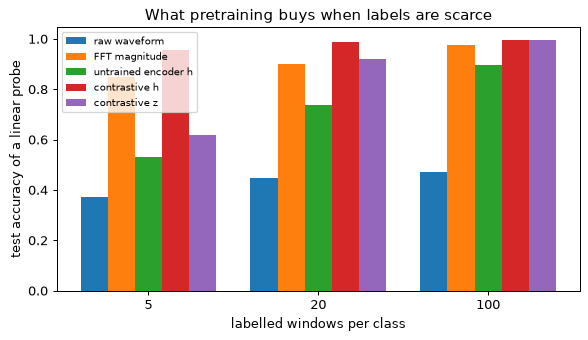
Read the table by columns. With 5 labels per class, the pretrained \mathbf{h} scores 0.956, against 0.850 for the FFT magnitudes, 0.532 for the untrained encoder and 0.371 for the raw waveform: eleven points above the classical feature, from a network that never saw a label during pretraining. The other two seeds give 0.954 and 0.944, so the margin does not depend on one lucky initialisation. With 100 labels per class the advantage has nearly gone (0.996 against 0.974): once labels are plentiful, a good hand-made feature is enough, and what pretraining buys is label efficiency. The projection output \mathbf{z} is a different story: at 5 labels it reaches only 0.620, far below \mathbf{h}, and at 100 it catches up. The head was trained to be invariant to whatever the augmentations vary, and it throws away more than the class needs; this is why SimCLR keeps \mathbf{h} and discards the head. The error bars of this protocol are not small (five draws of labelled windows, three pretraining seeds), so a difference of a point or two between rows should not be read as a ranking.
Step 7: the augmentations are the supervision
The last experiment removes augmentations. First the time shift only (gain and noise remain), then all three. Without the shift, the two views of a window have the same phases, so the easiest way to match them is to remember phase-dependent details of the waveform, which is exactly the feature that is useless for the classes. The loss still goes down, since the task is still solved, but it is solved by the wrong features. The confusion matrix of the no-shift model with 100 labels per class shows which classes pay.
model_noshift, loss_noshift = pretrain(seed=0, shift=False)
model_noaug, loss_noaug = pretrain(seed=0, shift=False, gain=False, noise=False)
ablation = {}
for name, m in [("no time shift", model_noshift), ("no augmentation", model_noaug)]:
    hp, _ = embed(m, X_pool)
    ht, _ = embed(m, X_test)
    ablation[name] = probe(hp, ht, return_model=True)
    print(f"{name:<22s}{fmt(ablation[name][0])}")
print(f"{'with all three':<22s}{fmt(acc_h)}")
print(f"final losses: full {np.mean(losses_full[-15:]):.3f}, "
      f"no shift {np.mean(loss_noshift[-15:]):.3f}, none {np.mean(loss_noaug[-15:]):.3f}")

pred = ablation["no time shift"][1]
cm = confusion_matrix(y_test, pred)
print("confusion matrix of the no-shift model (100 labels per class; rows = true):")
print(cm)
print(f"misalignment predicted as imbalance: {cm[2, 1]} of {cm[2].sum()}")
print(f"bearing defect predicted as healthy: {cm[3, 0]} of {cm[3].sum()}")
no time shift         0.622  0.809  0.977
no augmentation       0.581  0.747  0.942
with all three        0.956  0.988  0.996
final losses: full 2.376, no shift 1.746, none 1.692
confusion matrix of the no-shift model (100 labels per class; rows = true):
[[503   0   0   3]
 [  0 531   0   0]
 [  0  18 454   1]
 [ 13   0   0 477]]
misalignment predicted as imbalance: 18 of 473
bearing defect predicted as healthy: 13 of 490
Two observations. Without the time shift the probe accuracy at 5 labels per class falls from 0.956 to 0.622, which is about 0.09 above the untrained encoder’s 0.532 and far below the shifted model; with no augmentation at all it is 0.581. At 100 labels the gap closes to under 2 points (0.977 against 0.996), so the damage is again one of label efficiency: the features are usable but they are not organised by class. The final losses are the more instructive numbers: 1.75 without the shift and 1.69 with no augmentation, both lower than the 2.38 of the full recipe. The task of matching two views is easier when the views share their phases, so the loss improves while the representation gets worse. A contrastive loss measures how well the encoder solves the pretext task, not how good the features are for the downstream one, which is why the probe, and not the loss, decides. The confusion matrix of the no-shift model (one probe, one draw of 100 labels per class) puts the errors where the physics predicts: misalignment windows taken for imbalance (18 of 473), both of which have strong low harmonics, and bearing defects taken for healthy (13 of 490), whose impulses are small compared with the harmonics. These counts depend on the draw; the pattern, not the digits, is the point.
What you should see
- A linear classifier on the raw waveform is near chance for four classes at 5 labels per class (0.37, chance 0.25) and reaches only 0.47 at 100: with random phases no fixed linear combination of samples identifies a class. Spectral magnitudes, the classical feature, remove phase by construction and do well (0.85 rising to 0.97).
- Contrastive pretraining with a time-shift augmentation learns a phase-invariant representation without labels. With 5 labels per class it reaches 0.956, about eleven points above the FFT features, and two other pretraining seeds give 0.95 and 0.94; with 100 labels the two are within 2.5 points.
- The augmentation is the supervision. Without the time shift, the 5-label accuracy falls to 0.62, only a little above an untrained encoder (0.53), although the pretraining loss is lower (1.75 against 2.38). A lower contrastive loss does not mean better features.
- The projection head absorbs what the augmentations vary: probing \mathbf{z} with 5 labels per class gives 0.62 against 0.956 for \mathbf{h}, which is why \mathbf{h} is kept.
- The InfoNCE loss ends at about 2.4, well above zero and well below \log(2B - 1) = 6.24, the value for embeddings that carry no information.
Try this
- A wider gain augmentation. Replace the gain range 0.8 to 1.25 by 0.25 to 4 and probe \mathbf{h} again. The probe barely changes (a copy of this lab with the wider range gave 0.956, 0.990 and 0.997 for 5, 20 and 100 labels, against 0.956, 0.988 and 0.996), because healthy and imbalance windows also differ in harmonic ratios and in signal-to-noise ratio, so amplitude is not the only cue. Design an augmentation that does destroy a class distinction in these data, and confirm it with the confusion matrix. This is the conceptual failure of Section 11, the 6 and the 9 under rotation, made concrete.
- Temperature and batch size. Vary \tau over 0.05, 0.5 and 1.0 and the batch size over 64 and 512, keeping the number of epochs. Which settings change the probe’s 5-label accuracy, and does the final loss predict that?
- A class the encoder has never seen. Add a fifth class to the test set only, mechanical looseness (many harmonics of f_r with decaying amplitudes), and plot a two-dimensional PCA of \mathbf{h} for the test windows, coloured by class. Does the pretrained \mathbf{h} separate the new class from the old without any retraining? Compare with the PCA of the FFT magnitudes.
Exercises
Fifteen exercises follow the order of the sections they practise. They are graded by effort: ★ is conceptual and takes about 5 minutes, with at most a ratio or a sum to read off; ★★ is a derivation or a calculation and takes 10 to 12 minutes; ★★★ is coding and takes about 25 minutes. There are eight of the first kind, six of the second and one of the third, 127 minutes in all. Do the conceptual ones in your head or on paper first and only then open the solution: they are short because the whole difficulty is in committing to an answer.
None of the exercises reuses the numbers or the cases of a worked example, an inline check or a lab. The sections teach each method on one set of numbers; here the same method meets a different set, so that what transfers is the method and not the answer. Where a solution quotes a number, it was computed, and the code that produced it is shown or described. The one coding exercise (Exercise 12) starts from the physics-informed network of Lab 4 and is self-contained: its code runs as printed in one fresh Python session.
Every solution is hidden until you open it. Open one only after you have written your own answer, however rough: the check that matters is the place where your answer and the solution part ways.
An autoencoder maps 64-pixel images to a 128-dimensional code and back, with no other constraint, and its training reconstruction error reaches zero. Explain why the code is useless as a representation, and name two changes that would force the network to learn the structure of the data.
Show solution
Why zero error says nothing. Reconstruction error measures whether the output equals the input. It does not measure whether the code selected anything. Here the code has more dimensions than the input (d_z = 128 > d_x = 64), so the network is free to copy. One explicit solution: let the encoder place the 64 pixels in the first 64 code coordinates and zeros in the other 64, \mathbf{z} = (\mathbf{x}, \mathbf{0}), and let the decoder read the first 64 back. Any invertible map would do as well: a random rotation of \mathbf{x} and its inverse reconstruct perfectly, and the code is then a scrambled copy of the pixels. Gradient descent finds one of these because they are the easiest way to drive the loss to zero, and nothing in the objective prefers another.
The code is then useless in the three ways Section 2 lists. It has not compressed anything (128 numbers for 64). It has not separated likely inputs from unlikely ones, because the map is defined, and exact, for every input in \mathbb{R}^{64}, including noise. And it fails as an anomaly detector: an input the model has never seen is reconstructed as well as any other, so the reconstruction error, the anomaly score, is zero for everything.
Two changes that remove the identity from the set of minimisers.
- A bottleneck, d_z < d_x. A code with fewer numbers than the input cannot copy it. The network must decide which directions of variation to keep, and for squared error it keeps those that carry most of the variance (for linear maps the optimum spans the leading principal subspace, as Section 2 shows). The structure it learns is “where the data lie”.
- A denoising objective: corrupt the input to \tilde{\mathbf{x}} and ask for the clean \mathbf{x}. The identity now gives \tilde{\mathbf{x}}, which is wrong by the noise. The best possible map is the conditional mean \mathbb{E}[\mathbf{x}\mid\tilde{\mathbf{x}}], which pulls a corrupted point back towards where clean data are dense, and that is exactly what must be learnt about the data. Overcomplete codes then become harmless. (This is the same regression that Section 5 turns into the diffusion objective.)
Two further changes work for the same reason. A sparsity penalty on \mathbf{z} (an L1 term) lets many coordinates exist but allows few to be active, so the code cannot carry a dense copy. The variational autoencoder’s KL term (Section 3) charges nats for every bit of information the code carries about \mathbf{x}, so copying is expensive and only information that pays for itself in reconstruction survives.
The pattern: an autoencoder learns structure only to the extent that the architecture or the objective stops it from learning the identity. A low training error is therefore never the evidence that the representation is good; test it on corrupted, held-out or anomalous inputs.
(a) Starting from \log p_\theta(\mathbf{x}) = \log \int p_\theta(\mathbf{x}\mid\mathbf{z})\,p(\mathbf{z})\,d\mathbf{z}, insert q_\phi(\mathbf{z}\mid\mathbf{x})/q_\phi(\mathbf{z}\mid\mathbf{x}), apply Jensen’s inequality and obtain the ELBO \mathbb{E}_q[\log p_\theta(\mathbf{x}\mid\mathbf{z})] - D_{\KL}(q_\phi(\mathbf{z}\mid\mathbf{x}) \,\|\, p(\mathbf{z})).
(b) Without Jensen, show that \log p_\theta(\mathbf{x}) - \text{ELBO} = D_{\KL}(q_\phi(\mathbf{z}\mid\mathbf{x}) \,\|\, p_\theta(\mathbf{z}\mid\mathbf{x})), and say when the bound is tight.
(c) Show that D_{\KL}(\mathcal{N}(\mu, \sigma^2) \,\|\, \mathcal{N}(0, 1)) = \tfrac12(\mu^2 + \sigma^2 - \log\sigma^2 - 1), and that for a diagonal Gaussian the KL is a sum over dimensions. Evaluate it for \boldsymbol{\mu} = (0.3, -1.5, 0.0) and \boldsymbol{\sigma} = (0.8, 1.0, 2.0), and say what each dimension pays for.
Show solution
Write q for q_\phi(\mathbf{z}\mid\mathbf{x}) throughout, and assume q is positive wherever p_\theta(\mathbf{x}\mid\mathbf{z})p(\mathbf{z}) is, so that the division below is defined.
(a) The bound by Jensen. Multiplying and dividing by q changes nothing, and turns the integral into an expectation under q, a distribution we can sample:
The logarithm is concave, so Jensen’s inequality gives \log \mathbb{E}[Y] \ge \mathbb{E}[\log Y] for a positive random variable Y. Taking Y to be the ratio inside the brackets,
The last expectation is D_{\KL}(q \,\|\, p(\mathbf{z})) by definition, which is the stated ELBO. We moved the logarithm inside the expectation, which is the step that costs us equality: it replaces a quantity we cannot estimate without bias with one we can estimate from samples of \mathbf{z}.
(b) The gap, exactly. Bayes’ rule for the model, p_\theta(\mathbf{x}) = p_\theta(\mathbf{x}\mid\mathbf{z})\,p(\mathbf{z})\,/\,p_\theta(\mathbf{z}\mid\mathbf{x}), holds for every \mathbf{z}. Take logarithms and write the right-hand side as a product of two ratios by multiplying and dividing by q:
The left side does not depend on \mathbf{z}, so its expectation under any q is itself. Taking \mathbb{E}_q of both sides:
The first term is the ELBO by the algebra of part (a). So \log p_\theta(\mathbf{x}) - \text{ELBO} = D_{\KL}(q \,\|\, p_\theta(\mathbf{z}\mid\mathbf{x})) \ge 0, which proves the bound again without Jensen, and shows what Jensen threw away. A KL divergence is zero exactly when its two arguments are equal, so the bound is tight if and only if q_\phi(\mathbf{z}\mid\mathbf{x}) = p_\theta(\mathbf{z}\mid\mathbf{x}), the true posterior. Two consequences follow. Maximising the ELBO over \phi with \theta fixed is the same as minimising the KL to the true posterior, since \log p_\theta(\mathbf{x}) does not depend on \phi. And the gap is a property of the encoder family: a diagonal Gaussian q cannot match a posterior with two modes or correlated coordinates, however well it is trained.
(c) The Gaussian KL. For q = \mathcal{N}(\mu, \sigma^2) and p = \mathcal{N}(0, 1) in one dimension, the two log densities are
The KL is \mathbb{E}_q[\log q - \log p]. The \tfrac12\log 2\pi terms cancel. Under q, \mathbb{E}[(z-\mu)^2] = \sigma^2 (the definition of the variance) and \mathbb{E}[z^2] = \mu^2 + \sigma^2 (variance plus squared mean). Hence
For a diagonal Gaussian, q(\mathbf{z}) = \prod_j q_j(z_j) and p(\mathbf{z}) = \prod_j p_j(z_j), so \log q - \log p = \sum_j(\log q_j - \log p_j). The expectation of a sum is the sum of the expectations, and each term depends on one coordinate only, so only its marginal matters: D_{\KL}(q\,\|\,p) = \sum_j D_{\KL}(q_j \,\|\, p_j).
Numbers. Dimension by dimension, with \log\sigma^2 = 2\log\sigma:
- j = 1: \tfrac12(0.09 + 0.64 - \log 0.64 - 1) = \tfrac12(0.09 + 0.64 + 0.4463 - 1) = \tfrac12(0.1763) = 0.0881;
- j = 2: \tfrac12(2.25 + 1 - 0 - 1) = \tfrac12(2.25) = 1.1250;
- j = 3: \tfrac12(0 + 4 - \log 4 - 1) = \tfrac12(4 - 1.3863 - 1) = \tfrac12(1.6137) = 0.8069.
The total is 0.0881 + 1.1250 + 0.8069 = 2.020 nats. As a check, a Monte Carlo estimate of \mathbb{E}_q[\log q - \log p] from two million samples of \mathbf{z} gave 2.0196, within sampling error of the closed form.
What each dimension pays for. Split every term into its mean part \tfrac12\mu^2 and its width part \tfrac12(\sigma^2 - \log\sigma^2 - 1), which is zero at \sigma = 1 and positive on either side of it:
| dimension | mean part | width part | what it says about \mathbf{x} |
|---|---|---|---|
| 1 | 0.0450 | 0.0431 | little: close to the prior, slightly narrower |
| 2 | 1.1250 | 0 | a lot, in the position: the mean sits 1.5 prior standard deviations from 0 |
| 3 | 0 | 0.8069 | width only: the posterior is wider than the prior |
Dimension 2 is the typical informative coordinate: it pays for moving its mean away from the prior. Dimension 3 is the surprise. A posterior wider than the prior carries no information about \mathbf{x} in its mean, yet it costs 0.81 nats, because the KL penalises any departure from \mathcal{N}(0, 1), and a very diffuse q is a departure. In practice an encoder is pushed to \sigma \approx 1 and \mu \approx 0 for every coordinate it does not need, which is how posterior collapse looks in the numbers.
A VAE with d_z = 8 reports these per-dimension KL values on the test set, in nats: (2.1, 1.7, 0.003, 0.002, 1.2, 0.001, 0.004, 0.002). How many latent dimensions carry information about \mathbf{x}? What does the decoder do with the rest? Name two changes you would try if the task needs more of them.
Show solution
Three dimensions carry information: 1, 2 and 5. A per-dimension KL is the price in nats of the departure of q(z_j\mid\mathbf{x}) from the prior \mathcal{N}(0, 1), averaged over the test inputs (Exercise 2 shows the price for one coordinate). A price of 0.001 to 0.004 nats means that q(z_j\mid\mathbf{x}) is, for every input, essentially \mathcal{N}(0, 1): the mean does not move with \mathbf{x} and the width stays at 1. Together the three active dimensions use 2.1 + 1.7 + 1.2 = 5.0 nats, against 0.012 nats for the other five, so the code spends 99.8% of its budget on three coordinates. For scale, 5.0 nats is 7.2 bits, the most that the average input’s code can tell the decoder about it (the average KL is an upper bound on the information the code carries about \mathbf{x}).
What the decoder does with the rest. In those five coordinates z_j is a fresh draw from the prior, whatever the input: pure noise, independent of \mathbf{x}. Noise can only hurt reconstruction, so the decoder learns to ignore these inputs, with weights from them shrinking towards zero. This is partial posterior collapse: the coordinates are there but unused. Test it directly by decoding the same active code with different values of an inactive coordinate; the output should not change.
Whether it is a problem depends on the task. If the data really vary along three factors, three active dimensions is a good answer and the other five are free capacity. It is a problem only if reconstruction or sampling is poor in ways that more information would fix. Two changes to try, in the order of the cheapest first:
- Weaken the pressure of the KL term: a KL weight below 1, or a warm-up that ramps it from 0 to 1 over the first epochs so the decoder starts using the code before the penalty bites. A related device is free bits, which gives each coordinate a floor of nats below which the KL is not charged.
- Make reconstruction worth more, or the decoder less self-sufficient. A Gaussian decoder whose variance is large relative to the data makes errors cheap and information expensive; a summed squared error is that likelihood with \sigma_x^2 = \tfrac12 (Section 3), so a smaller variance (or a Bernoulli likelihood for pixels in [0, 1]) raises the exchange rate in favour of reconstruction. Separately, a smaller or less autoregressive decoder cannot model \mathbf{x} without the code, so it must use it.
Neither guarantees that an unused coordinate becomes useful. Measure the result by what you needed in the first place, for instance a held-out ELBO or the accuracy of a probe on the code, and not by the number of active dimensions.
(a) For fixed G, the GAN value is V = \int\big[p_{\text{data}}(\mathbf{x})\log D(\mathbf{x}) + p_g(\mathbf{x})\log(1 - D(\mathbf{x}))\big]\,d\mathbf{x}. Maximise the integrand pointwise to obtain D^*(\mathbf{x}).
(b) Substitute D^* and show that V(G, D^*) = -\log 4 + 2\,\mathrm{JSD}(p_{\text{data}} \,\|\, p_g), where \mathrm{JSD}(p \,\|\, q) = \tfrac12 D_{\KL}(p \,\|\, m) + \tfrac12 D_{\KL}(q \,\|\, m) and m = (p + q)/2.
(c) Check the result on three points with p_{\text{data}} = (0.6, 0.3, 0.1) and p_g = (0.2, 0.3, 0.5).
Show solution
(a) The optimal discriminator. The integral is a sum of independent integrands, one for each \mathbf{x}, and D is a free function, so the maximum over D is found by maximising each integrand separately over the number y = D(\mathbf{x}) \in (0, 1). Write a = p_{\text{data}}(\mathbf{x}) and b = p_g(\mathbf{x}), both positive, and f(y) = a\log y + b\log(1 - y). Then
The second derivative, f''(y) = -a/y^2 - b/(1-y)^2, is negative, so f is concave and the stationary point is its maximum. Hence
It is the posterior probability that \mathbf{x} is real, for a one-to-one mixture of real and generated points: the Bayes-optimal classifier.
(b) The value at the optimum. Substitute, using 1 - D^* = p_g/(p_{\text{data}} + p_g) and writing p = p_{\text{data}}, q = p_g:
With m = (p + q)/2 we have p + q = 2m, so \log\frac{p}{p+q} = \log\frac{p}{m} - \log 2, and likewise for q. The constants come out of the expectations (\mathbb{E}_p[1] = \mathbb{E}_q[1] = 1):
By the definition of the JSD the two KL terms sum to 2\,\mathrm{JSD}(p\,\|\,q), so V(G, D^*) = -\log 4 + 2\,\mathrm{JSD}(p_{\text{data}}\,\|\,p_g). The JSD is non-negative and zero only for equal distributions, so the generator’s best value is -\log 4 = -1.3863, reached at p_g = p_{\text{data}}. This is the sense in which a GAN, with a perfect discriminator, minimises a divergence. The proviso is the whole story of GAN training difficulty: the discriminator is never perfect, and when it is nearly perfect its gradients to the generator vanish (Section 4).
(c) The check.
Optimal discriminator. D^* = \big(\tfrac{0.6}{0.8}, \tfrac{0.3}{0.6}, \tfrac{0.1}{0.6}\big) = (0.75, 0.5, 0.1667).
Value. The data term is 0.6\log 0.75 + 0.3\log 0.5 + 0.1\log 0.1667 = -0.1726 - 0.2079 - 0.1792 = -0.5597. The generator term, with 1 - D^* = (0.25, 0.5, 0.8333), is 0.2\log 0.25 + 0.3\log 0.5 + 0.5\log 0.8333 = -0.2773 - 0.2079 - 0.0912 = -0.5764. So V = -1.1361.
Through the JSD. m = (0.4, 0.3, 0.3). D_{\KL}(p\,\|\,m) = 0.6\log\tfrac{0.6}{0.4} + 0.3\log 1 + 0.1\log\tfrac{0.1}{0.3} = 0.2433 + 0 - 0.1099 = 0.1334, and D_{\KL}(q\,\|\,m) = 0.2\log\tfrac{0.2}{0.4} + 0 + 0.5\log\tfrac{0.5}{0.3} = -0.1386 + 0.2554 = 0.1168. So \mathrm{JSD} = \tfrac12(0.1334 + 0.1168) = 0.1251, and -1.3863 + 2(0.1251) = -1.1361. The two routes agree to four decimals.
The value lies between the extremes -\log 4 = -1.3863 (identical distributions) and 0 (disjoint supports, where D^* separates real from generated perfectly), as it must. A short script reproduces all of these numbers.
import numpy as np

p = np.array([0.6, 0.3, 0.1])        # p_data
q = np.array([0.2, 0.3, 0.5])        # p_g
d_star = p / (p + q)
value = (p * np.log(d_star)).sum() + (q * np.log(1 - d_star)).sum()
m = (p + q) / 2
jsd = 0.5 * (p * np.log(p / m)).sum() + 0.5 * (q * np.log(q / m)).sum()
print("D* =", d_star.round(4))
print(f"V = {value:.4f}   -log 4 + 2 JSD = {-np.log(4) + 2 * jsd:.4f}   JSD = {jsd:.4f}")
D* = [0.75   0.5    0.1667]
V = -1.1361   -log 4 + 2 JSD = -1.1361   JSD = 0.1251
A GAN trained on cross-section images of turbine blades produces samples an engineer cannot tell from real ones, and its discriminator’s accuracy hovers around 50%. Describe one measurement that would reveal mode collapse: what you compute, what you compare it with, and what result would indicate collapse. Then explain why the discriminator’s 50% accuracy is no evidence against it.
Show solution
Measure coverage, not realism. Mode collapse is a failure of the generator to reach parts of p_{\text{data}}. A measurement that asks “do the samples look real?” is blind to it by construction, since each sample can look real and the samples can still be few. Ask instead whether the real data are near the samples.
- Describe every blade section by a vector: a feature embedding of the image from a network trained on something else, or, better for engineering use, a handful of geometric parameters (chord, thickness, camber, cooling-hole count). Do the same for a set of held-out real sections and for an equal number of generated ones.
- For each held-out real section, find the distance to its nearest generated sample (a recall-like distance).
- Compare it with a reference you can trust: the distance from each held-out real section to its nearest neighbour among an equally large set of other real sections. This reference says how close a perfect generator would get at this sample size, since a perfect generator draws from the same distribution.
- Also compute the precision-like distance, from each generated sample to its nearest real section, which is the realism measure.
What indicates collapse. The real-to-sample distances are much larger than the real-to-real reference, and the excess is concentrated: a block of real sections (a family of blades) has no generated sample anywhere near it. A summary that survives a skewed distribution is the fraction of real sections whose distance to the samples exceeds, say, the 99th percentile of the reference distances. For a generator that covers the data this fraction is about 1%, by the definition of the percentile. Realism, the precision-like distance, stays small throughout, which is why a realism metric or a human judge cannot detect the problem.
A constructed illustration, which is not a measurement of any real GAN: take eight kinds of section as eight tight clusters on a ring, a generator that samples only three of them perfectly, and a generator that covers all eight.
import numpy as np
from scipy.spatial import cKDTree

rng = np.random.default_rng(0)
angles = 2 * np.pi * np.arange(8) / 8
centres = 2.0 * np.stack([np.cos(angles), np.sin(angles)], axis=1)   # 8 kinds of section

def draw(n, kinds):
    k = rng.choice(kinds, size=n)
    return centres[k] + 0.1 * rng.standard_normal((n, 2))

train_real = draw(2000, range(8))           # stands in for the real sections
held_out = draw(1000, range(8))             # held-out real sections
full = draw(1000, range(8))                 # a generator that covers every kind
collapsed = draw(1000, [0, 3, 5])           # perfect samples, but only 3 kinds

def median_nn(queries, reference):
    return np.median(cKDTree(reference).query(queries)[0])

print(f"real -> real (reference)   {median_nn(held_out, train_real[:1000]):.3f}")
d_ref = cKDTree(train_real[:1000]).query(held_out)[0]
for name, gen in (("covering generator", full), ("collapsed generator", collapsed)):
    d_gen = cKDTree(gen).query(held_out)[0]
    uncovered = np.mean(d_gen > np.quantile(d_ref, 0.99))
    print(f"{name}: sample->real {median_nn(gen, held_out):.3f}, "
          f"real->sample {median_nn(held_out, gen):.3f}, "
          f"uncovered real sections {uncovered:.3f}")
real -> real (reference)   0.016
covering generator: sample->real 0.016, real->sample 0.016, uncovered real sections 0.011
collapsed generator: sample->real 0.016, real->sample 1.141, uncovered real sections 0.621
The collapsed generator is as realistic as the covering one (0.016 both), yet 62% of the real sections lie beyond the reference distance from every sample; that is 5/8 = 62.5\%, the five clusters it never visits. The median real-to-sample distance jumped from 0.016 to 1.141 only because more than half of the data are uncovered: a collapse that misses a third of the data would leave the median unchanged, which is why the uncovered fraction is the better summary. The same samples-to-training-set distances also expose the opposite failure, near-copies of training images.
Why 50% discriminator accuracy proves nothing. The discriminator is trained to separate samples from data where the samples are. Regions of p_{\text{data}} that the generator never visits contribute nothing to the generator’s loss, since the generator is rewarded only for the samples it makes; and the discriminator sees no generated sample there to separate. Near 50% means that in the places the generator visits it is indistinguishable from the data. It says nothing about the places it does not. Moreover, the two networks play a game and not an optimisation: a discriminator that cycles, always chasing the generator’s current favourite mode, sits near 50% on average while the generator hops from one mode to the next (Section 4). The accuracy is a symptom of balance between two players, not of coverage.
Show that the per-step forward process q(\mathbf{x}_t\mid\mathbf{x}_{t-1}) = \mathcal{N}\big(\sqrt{1-\beta_t}\,\mathbf{x}_{t-1},\ \beta_t\mathbf{I}\big) gives q(\mathbf{x}_t\mid\mathbf{x}_0) = \mathcal{N}\big(\sqrt{\bar\alpha_t}\,\mathbf{x}_0,\ (1-\bar\alpha_t)\mathbf{I}\big) with \bar\alpha_t = \prod_{s\le t}(1-\beta_s). Write \mathbf{x}_t = \sqrt{\alpha_t}\,\mathbf{x}_{t-1} + \sqrt{1-\alpha_t}\,\boldsymbol{\epsilon}_t, assume the result for t - 1, and use the fact that a sum of independent zero-mean Gaussians is Gaussian with the sum of the variances.
Show solution
The set-up. With \alpha_t = 1 - \beta_t, sampling from \mathcal{N}(\sqrt{\alpha_t}\,\mathbf{x}_{t-1}, \beta_t\mathbf{I}) is the same as the stated one-line update with fresh \boldsymbol{\epsilon}_t \sim \mathcal{N}(\mathbf{0}, \mathbf{I}), independent of everything before step t: scaling a standard normal by \sqrt{\beta_t} = \sqrt{1-\alpha_t} gives variance \beta_t, and adding the mean shifts it. We prove the claim by induction on t, with the statement “\mathbf{x}_t = \sqrt{\bar\alpha_t}\,\mathbf{x}_0 + \sqrt{1-\bar\alpha_t}\,\bar{\boldsymbol{\epsilon}}_t for some \bar{\boldsymbol{\epsilon}}_t \sim \mathcal{N}(\mathbf{0}, \mathbf{I}) that is independent of the later noises \boldsymbol{\epsilon}_{t+1}, \boldsymbol{\epsilon}_{t+2}, \dots”. Independence from later noise is what the step needs.
Base case, t = 1. \mathbf{x}_1 = \sqrt{\alpha_1}\,\mathbf{x}_0 + \sqrt{1-\alpha_1}\,\boldsymbol{\epsilon}_1, and \bar\alpha_1 = \alpha_1, so the statement holds with \bar{\boldsymbol{\epsilon}}_1 = \boldsymbol{\epsilon}_1.
Induction step. Assume the statement for t - 1 and substitute it into the update for step t:
Since \alpha_t\bar\alpha_{t-1} = \bar\alpha_t, the mean is \sqrt{\bar\alpha_t}\,\mathbf{x}_0. The noise is a sum of two independent zero-mean Gaussian vectors (\bar{\boldsymbol{\epsilon}}_{t-1} is independent of \boldsymbol{\epsilon}_t by the induction hypothesis), with covariances \alpha_t(1-\bar\alpha_{t-1})\mathbf{I} and (1-\alpha_t)\mathbf{I}. Their sum is Gaussian with zero mean and covariance
A zero-mean Gaussian with covariance (1-\bar\alpha_t)\mathbf{I} can be written \sqrt{1-\bar\alpha_t}\,\bar{\boldsymbol{\epsilon}}_t with \bar{\boldsymbol{\epsilon}}_t \sim \mathcal{N}(\mathbf{0}, \mathbf{I}), and \bar{\boldsymbol{\epsilon}}_t is built from \bar{\boldsymbol{\epsilon}}_{t-1} and \boldsymbol{\epsilon}_t only, so it is independent of \boldsymbol{\epsilon}_{t+1}, \dots. That completes the induction, and gives
Why the step works. The key identity is \alpha_t(1-\bar\alpha_{t-1}) + (1-\alpha_t) = 1 - \alpha_t\bar\alpha_{t-1}: the variance that earlier noise has acquired, shrunk by the factor \alpha_t the signal is scaled by, plus the fresh noise of this step, is exactly what is missing from the signal’s shrinking weight. That the squares of the two scales sum to 1 at every t is the reason the process keeps unit-variance data at unit variance.
A numerical check. Take three steps with \beta = (0.1, 0.2, 0.3) (exaggerated, so the numbers are visible), so \alpha = (0.9, 0.8, 0.7) and \bar\alpha = (0.9,\ 0.72,\ 0.504). For a fixed \mathbf{x}_0 the variance of \mathbf{x}_t obeys \mathrm{Var}_t = \alpha_t\mathrm{Var}_{t-1} + \beta_t. The recursion gives 0.1, then 0.8 \times 0.1 + 0.2 = 0.28, then 0.7 \times 0.28 + 0.3 = 0.496, which equal 1 - \bar\alpha_t = 0.1, 0.28, 0.496 as the formula says.
import numpy as np

beta = np.array([0.1, 0.2, 0.3])
alpha = 1 - beta
alpha_bar = np.cumprod(alpha)

var = 0.0
for t in range(3):
    var = alpha[t] * var + beta[t]       # variance recursion for fixed x_0
    print(f"t={t + 1}: recursion {var:.4f}   1 - alpha_bar {1 - alpha_bar[t]:.4f}")

rng = np.random.default_rng(0)
x = np.ones(1_000_000)                   # one million chains started at x_0 = 1
for t in range(3):
    x = np.sqrt(alpha[t]) * x + np.sqrt(beta[t]) * rng.standard_normal(x.size)
print(f"sampled mean {x.mean():.4f} (sqrt(alpha_bar) = {np.sqrt(alpha_bar[2]):.4f}), "
      f"sampled variance {x.var():.4f}")
t=1: recursion 0.1000   1 - alpha_bar 0.1000
t=2: recursion 0.2800   1 - alpha_bar 0.2800
t=3: recursion 0.4960   1 - alpha_bar 0.4960
sampled mean 0.7097 (sqrt(alpha_bar) = 0.7099), sampled variance 0.4953
Running the chain a million times gives mean 0.7097 against \sqrt{0.504} = 0.7099 and variance 0.4953 against 0.496, as the closed form predicts (the last digits are sampling noise).
Ho et al.'s linear schedule runs \beta_t evenly from 10^{-4} to 0.02 over T = 1000 steps.
(a) Estimate \bar\alpha_T using \log(1-\beta) \approx -\beta and compare with the exact product, 4.04\times10^{-5}.
(b) Someone keeps the same \beta range but sets T = 100. Estimate \bar\alpha_T and \sqrt{\bar\alpha_T}.
(c) Explain what goes wrong when that model is sampled from \mathbf{x}_T \sim \mathcal{N}(\mathbf{0}, \mathbf{I}), and give two fixes.
Show solution
The tool. \bar\alpha_T = \prod_t(1-\beta_t), so \log\bar\alpha_T = \sum_t\log(1-\beta_t). The series \log(1-\beta) = -\beta - \tfrac12\beta^2 - \dots shows that for small \beta the first term dominates, and \bar\alpha_T \approx \exp(-\sum_t\beta_t).
(a) The \beta_t are an arithmetic sequence, so their sum is the number of terms times the mean of the endpoints: 1000 \times (10^{-4} + 0.02)/2 = 1000 \times 0.01005 = 10.05. Then \bar\alpha_T \approx e^{-10.05} = 4.32\times10^{-5}, within 7% of the exact 4.04\times10^{-5}. Most of the difference is the next term of the series. \sum_t\beta_t^2/2 = 0.067 here, so \bar\alpha_T \approx e^{-10.05 - 0.067} = 4.04\times10^{-5}, which matches to three figures. The signal amplitude left at the last step is \sqrt{\bar\alpha_T} = 0.0064: not zero, but about 0.6% of the signal, which is small enough for the model to be sampled from pure noise.
(b) With T = 100 the same range gives \sum_t\beta_t = 100 \times 0.01005 = 1.005, so \bar\alpha_T \approx e^{-1.005} = 0.366. The exact product is 0.364 (the correction is now only \sum\beta^2/2 = 0.0067). So \sqrt{\bar\alpha_T} \approx 0.60: at the noisiest step 60% of the signal amplitude remains, and \mathbf{x}_T is far from \mathcal{N}(\mathbf{0}, \mathbf{I}). The schedule was designed for ten times as many steps; each step adds a fixed small amount of noise, and with a tenth of them the total falls far short.
(c) What goes wrong. Sampling starts from \mathbf{x}_T \sim \mathcal{N}(\mathbf{0}, \mathbf{I}), a signal-free draw. But during training the network was shown, at t = T, inputs \mathbf{x}_T = 0.60\,\mathbf{x}_0 + 0.80\,\boldsymbol{\epsilon}, which still contain a clear signal. At the first reverse step the network meets an input distribution it was never trained on, a train–test mismatch, and its prediction of the noise is wrong in a systematic way: it expects to find \mathbf{x}_0 in the input, so it reads structure into noise, and the error propagates through all later steps. The effect has been documented for image models whose last step is not pure noise, which cannot generate very bright or very dark images because the mean brightness of the training signal leaks through the noise (Lin et al. 2024, in the references).
Two fixes.
- Rescale the schedule to the new T, so that \bar\alpha_T is again near 0: multiply the range by 1000/T = 10, giving \beta_t from 10^{-3} to 0.2. The sum is again 10.05 and the exact \bar\alpha_T = 2.0\times10^{-5}.
- Use a schedule built to end in noise, such as the cosine schedule, which at T = 100 gives \bar\alpha_T = 2.4\times10^{-7} (with \beta_T clipped at 0.999, as in the original), or rescale any schedule to zero terminal signal-to-noise ratio.
(Fewer steps also make each step bigger, so a coarse linear schedule loses accuracy in the reverse process; the rescaling fixes the endpoint, not the discretisation.)
import numpy as np

def report(name, beta):
    alpha_bar = np.prod(1 - beta)
    print(f"{name:34s} sum(beta) {beta.sum():6.3f}  e^-sum {np.exp(-beta.sum()):.3e}  "
          f"alpha_bar_T {alpha_bar:.3e}  sqrt {np.sqrt(alpha_bar):.4f}")

report("T=1000, 1e-4 to 0.02", np.linspace(1e-4, 0.02, 1000))
report("T=100,  1e-4 to 0.02", np.linspace(1e-4, 0.02, 100))
report("T=100,  rescaled 1e-3 to 0.2", np.linspace(1e-3, 0.2, 100))

T, s = 100, 0.008                        # cosine schedule, s = 0.008
t = np.arange(T + 1) / T
f = np.cos((t + s) / (1 + s) * np.pi / 2) ** 2
report("T=100, cosine (clip 0.999)", np.clip(1 - f[1:] / f[:-1], 0, 0.999))
T=1000, 1e-4 to 0.02               sum(beta) 10.050  e^-sum 4.319e-05  alpha_bar_T 4.036e-05  sqrt 0.0064
T=100,  1e-4 to 0.02               sum(beta)  1.005  e^-sum 3.660e-01  alpha_bar_T 3.636e-01  sqrt 0.6030
T=100,  rescaled 1e-3 to 0.2       sum(beta) 10.050  e^-sum 4.319e-05  alpha_bar_T 2.039e-05  sqrt 0.0045
T=100, cosine (clip 0.999)         sum(beta)  7.879  e^-sum 3.787e-04  alpha_bar_T 2.429e-07  sqrt 0.0005
Two cautions on reading the table. The e^{-\sum\beta} approximation is poor for the cosine row (its last \beta is 0.999, so the first-order series does not apply), which is why the exact product is the number to use. And a rescaled schedule with \beta up to 0.2 has large individual steps; it is the right endpoint, not necessarily the best path.
A gate with three basic-event inputs forms a star graph: centre c joined to leaves a, b and d.
(a) Write \hat{\mathbf{A}} = \tilde{\mathbf{D}}^{-1/2}(\mathbf{A} + \mathbf{I})\tilde{\mathbf{D}}^{-1/2}.
(b) With the scalar feature \mathbf{x} = (1, 0, 0, 0) (centre first), compute \hat{\mathbf{A}}\mathbf{x} and \hat{\mathbf{A}}^2\mathbf{x}.
(c) Find the limit of \hat{\mathbf{A}}^k\mathbf{x} as k grows, using the eigenvector \mathbf{u} \propto \tilde{\mathbf{D}}^{1/2}\mathbf{1}, and the ratio of the centre’s value to a leaf’s.
(d) The eigenvalues of \hat{\mathbf{A}} are 1, 0.5, 0.5 and -0.25, and the eigenvectors for 0.5 are zero at the centre and sum to zero over the leaves. How fast does \hat{\mathbf{A}}^k\mathbf{x} approach its limit for this \mathbf{x}, and why not as 0.5^k?
Show solution
(a) The matrix. Adding self-loops gives \tilde{\mathbf{A}} = \mathbf{A} + \mathbf{I}, with the centre joined to every node and every leaf to the centre and itself. The row sums are the degrees with self-loop: \tilde{d}_c = 1 + 3 = 4 and \tilde{d}_{\text{leaf}} = 1 + 1 = 2. Entry (i, j) of \hat{\mathbf{A}} is \tilde{A}_{ij}/\sqrt{\tilde{d}_i\tilde{d}_j}, so:
- centre to itself: 1/\sqrt{4\cdot4} = 1/4;
- centre to a leaf, and back: 1/\sqrt{4\cdot2} = 1/\sqrt8 = 0.3536;
- a leaf to itself: 1/\sqrt{2\cdot2} = 1/2;
- between two leaves: 0 (they are not adjacent).
(b) Two layers of propagation. \hat{\mathbf{A}}\mathbf{x} is the first column of \hat{\mathbf{A}}: (0.25,\ 0.3536,\ 0.3536,\ 0.3536). After one step the feature has reached every leaf, each with 0.3536, more than the centre’s own 0.25 (the centre’s value is divided by 4 but each leaf’s is divided by \sqrt8). Applying \hat{\mathbf{A}} again, row by row:
- centre: 0.25\times0.25 + 3\times(0.3536\times0.3536) = 0.0625 + 3\times0.125 = 0.4375;
- each leaf: 0.3536\times0.25 + 0.5\times0.3536 = 0.0884 + 0.1768 = 0.2652.
So \hat{\mathbf{A}}^2\mathbf{x} = (0.4375,\ 0.2652,\ 0.2652,\ 0.2652). The centre’s value swings up and down while the leaves settle.
(c) The limit. The vector \tilde{\mathbf{D}}^{1/2}\mathbf{1} is an eigenvector of \hat{\mathbf{A}} with eigenvalue 1:
because \tilde{\mathbf{A}}\mathbf{1} is the vector of row sums \tilde{\mathbf{d}} and \tilde{\mathbf{D}}^{-1/2}\tilde{\mathbf{d}} = \tilde{\mathbf{D}}^{1/2}\mathbf{1}. Here it is (2, \sqrt2, \sqrt2, \sqrt2); normalised to unit length (its squared norm is 4 + 6 = 10), \mathbf{u} = (2, \sqrt2, \sqrt2, \sqrt2)/\sqrt{10} = (0.6325, 0.4472, 0.4472, 0.4472).
\hat{\mathbf{A}} is symmetric, so its eigenvectors are orthogonal and \mathbf{x} decomposes into them. Every other eigenvalue has magnitude below 1 (they are 0.5, 0.5, -0.25), so after many applications only the component along \mathbf{u} survives: \hat{\mathbf{A}}^k\mathbf{x} \to \mathbf{u}\,(\mathbf{u}^\top\mathbf{x}). With \mathbf{u}^\top\mathbf{x} = 0.6325,
Its centre-to-leaf ratio is \sqrt{\tilde{d}_c/\tilde{d}_{\text{leaf}}} = \sqrt{4/2} = \sqrt2 = 1.414. In the limit the nodes differ only by the square root of their degree: whatever the input feature was, it has been washed out and what is left is how well connected each node is. This is over-smoothing in its purest form (Section 8).
(d) How fast. The error after k steps is \hat{\mathbf{A}}^k\mathbf{x} minus the limit, which is the part of \mathbf{x} orthogonal to \mathbf{u}, multiplied k times by the other eigenvalues. Decompose it:
The eigenvectors for 0.5 are zero at the centre and sum to zero over the leaves, so a vector that takes the same value on all three leaves has no component along them (its inner product with each is that value times the sum of the eigenvector’s leaf entries, which is 0). The remainder takes the value -0.2828 on all three leaves, so it lies entirely along the last eigenvector, for \lambda = -0.25: indeed (0.6, -0.2828, -0.2828, -0.2828) is proportional to (-2.121, 1, 1, 1), and one checks \hat{\mathbf{A}}\mathbf{v} = -0.25\,\mathbf{v} directly (centre row: 0.25(-2.121) + 3(0.3536) = 0.530 = -0.25(-2.121); leaf row: 0.3536(-2.121) + 0.5 = -0.25). So the error is multiplied by -0.25 at each step: it shrinks by a factor of 4 per step and flips sign, which is the swing seen in (b), where the centre went 0.25 \to 0.4375 \to 0.3906 \to 0.4023 \to \dots around 0.4. The relative errors \|\hat{\mathbf{A}}^k\mathbf{x} - \text{limit}\| / \|\text{limit}\| are 0.306,\ 0.0765,\ 0.0191,\ 0.0048 for k = 1, \dots, 4: below 1% from k = 4.
The second-largest eigenvalue magnitude (here 0.5) bounds the rate for any feature vector, but the actual rate is set by which eigenvectors the features touch. A leaf’s feature, \mathbf{x} = (0, 1, 0, 0), has a component along the \lambda = 0.5 eigenspace (it is (0, \tfrac23, -\tfrac13, -\tfrac13), of norm 0.8165, against a limit of norm 0.4472) and converges as 0.5^k: the relative error is 1.83 \times 0.5^k plus the -0.25 part, which gives 0.935 at k = 1, 0.114 at k = 4 and 0.0071 at k = 8, below 1% only from k = 8. Symmetric inputs converge fast; asymmetric ones are limited by the worst eigenvalue.
import numpy as np

A = np.zeros((4, 4))
A[0, 1:] = A[1:, 0] = 1                    # node 0 is the centre, 1-3 the leaves
A_tilde = A + np.eye(4)
d_tilde = A_tilde.sum(axis=1)              # (4, 2, 2, 2)
A_hat = A_tilde / np.sqrt(np.outer(d_tilde, d_tilde))
print("A_hat =\n", A_hat.round(4))
print("eigenvalues", np.linalg.eigvalsh(A_hat).round(4))

u = np.sqrt(d_tilde) / np.linalg.norm(np.sqrt(d_tilde))
for label, x in (("centre feature", np.array([1.0, 0, 0, 0])),
                 ("leaf feature  ", np.array([0, 1.0, 0, 0]))):
    limit = u * (u @ x)
    errors, h = [], x.copy()
    for k in range(1, 9):
        h = A_hat @ h
        errors.append(np.linalg.norm(h - limit) / np.linalg.norm(limit))
    print(label, "limit", limit.round(4))
    print("   relative error, k = 1..8:", " ".join(f"{e:.4f}" for e in errors))
    if label.startswith("centre"):
        print("   A_hat x   =", (A_hat @ x).round(4))
        print("   A_hat^2 x =", (A_hat @ A_hat @ x).round(4))
A_hat =
 [[0.25   0.3536 0.3536 0.3536]
 [0.3536 0.5    0.     0.    ]
 [0.3536 0.     0.5    0.    ]
 [0.3536 0.     0.     0.5   ]]
eigenvalues [-0.25  0.5   0.5   1.  ]
centre feature limit [0.4    0.2828 0.2828 0.2828]
   relative error, k = 1..8: 0.3062 0.0765 0.0191 0.0048 0.0012 0.0003 0.0001 0.0000
   A_hat x   = [0.25   0.3536 0.3536 0.3536]
   A_hat^2 x = [0.4375 0.2652 0.2652 0.2652]
leaf feature   limit [0.2828 0.2    0.2    0.2   ]
   relative error, k = 1..8: 0.9354 0.4593 0.2286 0.1142 0.0571 0.0285 0.0143 0.0071
A colleague trains a two-layer GCN to predict which nodes of fault trees are basic events, with node degree among the features, and reports 99% test accuracy. What baseline should the result be compared with, what does that baseline score, and what task would actually test whether a GNN has learned something about fault-tree structure?
Show solution
The baseline is a one-line rule. In a fault tree the basic events are exactly the leaves, the nodes with no inputs below them. A leaf is joined to its parent gate only, so every non-top node with a single neighbour is a basic event. Every gate has at least two inputs plus a parent (or, for the top event, at least two inputs), so a gate always has at least two neighbours. Therefore “basic event if and only if the node has exactly one neighbour” is correct for every node of every fault tree: it scores 100%. A model with degree among its features is handed the answer: the classifier has only to threshold one input.
So 99% test accuracy is not evidence of anything. It is below the free baseline. The sensible comparison for any classification result starts with the cheapest rule that uses the same inputs, as in Module 01, and the number to report is the margin over it.
A short experiment makes the point. It generates 300 random fault trees (gates with two or three inputs, each input a basic event with probability 0.45 or a gate until a depth limit), scores the leaf rule, and trains a two-layer GCN with degree as the only feature on 200 trees, testing on the other 100: the split is by tree, never by node, since nodes of one tree share their structure (leakage, Module 01).
import numpy as np, torch, torch.nn as nn
rng = np.random.default_rng(0)
torch.manual_seed(0)

def random_fault_tree(max_depth=4):
    """Return (edges, is_basic_event). Node 0 is the top gate; gates have 2-3 inputs."""
    edges, is_basic, frontier = [], [False], [(0, 0)]
    while frontier:
        node, depth = frontier.pop()
        for _ in range(rng.integers(2, 4)):          # a gate has 2 or 3 inputs
            child = len(is_basic)
            leaf = depth + 1 >= max_depth or rng.random() < 0.45
            is_basic.append(bool(leaf))
            edges.append((node, child))
            if not leaf:
                frontier.append((child, depth + 1))
    return edges, np.array(is_basic)

def graph_tensors(edges, n):
    A = np.zeros((n, n), dtype=np.float32)
    for a, b in edges:
        A[a, b] = A[b, a] = 1.0
    At = A + np.eye(n, dtype=np.float32)
    dinv = 1.0 / np.sqrt(At.sum(1))
    return torch.tensor(dinv[:, None] * At * dinv[None, :]), A.sum(1)

trees = [random_fault_tree() for _ in range(300)]
data = []
for edges, basic in trees:
    n = len(basic)
    A_hat, deg = graph_tensors(edges, n)
    data.append((A_hat, torch.tensor(deg[:, None] / 4.0, dtype=torch.float32),
                 torch.tensor(basic, dtype=torch.float32)))
sizes = [len(b) for _, b in trees]
print("nodes per tree: min", min(sizes), "max", max(sizes))

# the baseline: a node with exactly one neighbour is a basic event
rule_correct = sum(int(((d[1].squeeze() == 0.25) == d[2].bool()).sum()) for d in data)
print(f"leaf rule accuracy: {rule_correct / sum(sizes):.4f}")

class GCN(nn.Module):
    def __init__(self, hidden=16):
        super().__init__()
        self.w1, self.w2 = nn.Linear(1, hidden), nn.Linear(hidden, 1)
    def forward(self, A_hat, x):
        h = torch.relu(A_hat @ self.w1(x))
        return (A_hat @ self.w2(h)).squeeze(-1)

train, test = data[:200], data[200:]            # split by tree, not by node
model = GCN()
opt = torch.optim.Adam(model.parameters(), lr=1e-2)
for epoch in range(300):
    for A_hat, x, y in train:
        loss = nn.functional.binary_cross_entropy_with_logits(model(A_hat, x), y)
        opt.zero_grad(); loss.backward(); opt.step()

def accuracy(split):
    ok = tot = 0
    with torch.no_grad():
        for A_hat, x, y in split:
            ok += int(((model(A_hat, x) > 0).float() == y).sum()); tot += len(y)
    return ok / tot

share = np.mean(np.concatenate([b for _, b in trees]))
print(f"GCN test accuracy: {accuracy(test):.4f}")
print(f"share of basic events (majority baseline): {max(share, 1 - share):.4f}")
nodes per tree: min 3 max 58
leaf rule accuracy: 1.0000
GCN test accuracy: 0.8306
share of basic events (majority baseline): 0.6237
(Last digits may differ between machines.) The leaf rule scores exactly 1.0000. The GCN, which receives the degree and averages it with its neighbours’ degrees at every layer, gets 0.83 here, well above the majority class (0.62) and well below the rule: the normalised aggregation blurs the one number that carries the answer, and the network has to learn to undo that. A different feature set or longer training moves it, but it cannot beat the rule, and it was never going to. Whatever the colleague’s 99% reflects, the correct reading is that a rule solves this task and the network approximates it.
A task that tests structure. Choose a label that needs information several hops away and is not a function of a node’s own neighbourhood size. The example of Lab 3 is single points of failure: a basic event whose failure alone brings down the top event, which happens when every gate on its path to the top is an OR gate. Whether a node qualifies depends on gate types all the way to the root, so a network with L layers sees only L hops of it. Evaluate with a split by tree, compare against simple baselines (the majority class; “the gate above is an OR”) and against the exact algorithm, and report the accuracy as a function of depth. That is a result that says something about whether message passing learned the structure.
Graph P is the complete bipartite graph K_{3,3}: two rows of three nodes, each node joined to all three nodes of the other row. Graph Q is the triangular prism: two triangles with corresponding corners joined. Every node has the same feature vector. Explain why any message-passing GNN (GCN, GAT, GIN) gives every node the same embedding in both graphs, whatever the number of layers, and why a sum or mean readout cannot tell P from Q. Propose one input feature that would.
Show solution
The two graphs look the same locally. Count: both have 6 nodes and 9 edges, and in both every node has exactly three neighbours (in K_{3,3} the three nodes of the other row; in the prism the two triangle neighbours and the partner corner). They are both 3-regular.
Why every node ends up with the same embedding. Take any layer of a message-passing network. A node’s new embedding is a function of its own current embedding and of the multiset of its neighbours’ embeddings. Initially all 12 nodes (6 in each graph) carry the same vector \mathbf{h}^{(0)}. By induction, suppose all nodes carry the same \mathbf{h}^{(l)}. Then every node receives the same three identical messages and applies the same update, so all carry the same \mathbf{h}^{(l+1)}. Concretely:
- GCN: the degree with self-loop is 4 for every node, every weight is 1/\sqrt{4\cdot4} = 1/4, and the new embedding is \phi\big(\tfrac14\mathbf{W}\mathbf{h} + 3\cdot\tfrac14\mathbf{W}\mathbf{h}\big), the same everywhere;
- GAT: the attention weights are a softmax over three neighbours whose keys are identical, hence uniform (1/3 each); the weighted sum of identical vectors is that vector;
- GIN: the sum of three identical vectors is three times that vector, again the same everywhere.
This holds for every layer, so any depth leaves all node embeddings identical, in both graphs and with the same value in P and in Q.
Why the readout cannot help. A sum readout over six identical vectors is 6\mathbf{h}^{(L)} and a mean is \mathbf{h}^{(L)}, the same for P as for Q. Nothing after the last layer sees anything but these identical embeddings.
The limit behind it. This is the 1-Weisfeiler–Lehman limit: colour refinement (repeatedly recolouring each node by its colour and the multiset of its neighbours’ colours) never splits the nodes of a regular graph, and message-passing networks are at most as discriminating as that test. Yet the graphs are different objects: the prism contains two triangles, while K_{3,3}, being bipartite, has no odd cycles and so no triangle. In a safety setting this is the difference between two redundancy structures that a message-passing network would score identically.
Features that break the tie (each adds information that message passing cannot compute for itself):
- the number of triangles through each node: 1 for every node of Q, 0 for every node of P (equivalently the diagonal of \mathbf{A}^3 divided by 2; \operatorname{tr}(\mathbf{A}^3)/6 is 2 triangles for Q, 0 for P);
- the length of the shortest cycle through the node: 3 against 4;
- random node identifiers, which break the symmetry at the cost of making the embeddings depend on the draw;
- a spectral positional encoding. The adjacency eigenvalues are 3, 0, 0, 0, 0, -3 for P and 3, 1, 0, 0, -2, -2 for Q, so even the spectrum separates them.
(The eigenvalues and triangle counts were computed with NumPy; \mathbf{A} of each graph has all row sums equal to 3.)
For u'' + 2\zeta\omega_0 u' + \omega_0^2 u = 0 with u(0) = 1 and u'(0) = 0, a student proposes the trial solution u(t) = e^{-\zeta\omega_0 t}\cos\omega_0 t: decaying, but at the undamped frequency.
(a) Compute the residual r(t) symbolically.
(b) Evaluate r(0) and the initial-condition terms (u(0) - 1)^2 and u'(0)^2 for \zeta = 0.1 and \omega_0 = 2\pi.
(c) What two changes give the exact solution, and how would a PINN’s loss report the trial function’s error?
Show solution
(a) The residual. Write a = \zeta\omega_0, so the equation is u'' + 2a\,u' + \omega_0^2 u = 0 and the trial is u = e^{-at}\cos\omega_0 t. Two derivatives with the product rule:
Substitute into r = u'' + 2a\,u' + \omega_0^2 u, factoring out e^{-at}:
The sine terms cancel (+2a\omega_0 from u'', -2a\omega_0 from 2a\,u'). The cosine coefficient is a^2 - \omega_0^2 - 2a^2 + \omega_0^2 = -a^2. So
The residual is of order \zeta^2: a trial that gets the decay right and the frequency slightly wrong is nearly a solution as far as the equation can tell. This is the key to part (c).
(b) The numbers. \zeta^2\omega_0^2 = 0.01 \times (2\pi)^2 = 0.3948, so
- r(0) = -0.3948 (the cosine and the exponential are both 1);
- u(0) = 1, so (u(0) - 1)^2 = 0;
- u'(0) = -a = -\zeta\omega_0 = -0.6283 (from the expression for u' with t = 0: -a\cdot1 - \omega_0\cdot0), so u'(0)^2 = 0.3948, which equals a^2.
(c) The exact solution, and what the loss says. The undamped frequency is the error. A solution of the form e^{-at}\cos\omega t has residual e^{-at}(\omega_0^2 - a^2 - \omega^2)\cos\omega t (the same algebra with \omega in place of \omega_0 in the trial’s own derivatives), which vanishes if and only if \omega^2 = \omega_0^2 - a^2 = \omega_0^2(1 - \zeta^2). The two changes are therefore:
- Replace \omega_0 by the damped frequency \omega_d = \omega_0\sqrt{1 - \zeta^2} = 6.252 rad/s inside the cosine. The result solves the equation exactly but still has u'(0) = -a \neq 0.
- Add the sine term \dfrac{\zeta\omega_0}{\omega_d}\,e^{-at}\sin\omega_d t. It is also a solution of the same linear equation (the algebra above, for the sine, gives zero residual by the same condition on \omega), so adding it keeps the residual at zero, and its derivative at 0 is +a, which cancels the -a: u'(0) = 0.
The result, u = e^{-at}\big[\cos\omega_d t + (\zeta\omega_0/\omega_d)\sin\omega_d t\big], is the exact solution of Section 9. A symbolic check confirms it: its residual simplifies to 0, u(0) = 1 and u'(0) = 0.
What a PINN’s loss reports for the trial. Three terms:
- Initial position: (u(0) - 1)^2 = 0.
- Initial velocity: u'(0)^2 = 0.395.
- Residual: the mean of r^2 over [0, 2] s. The integral of \zeta^4\omega_0^4 e^{-2at}\cos^2\omega_0 t over the interval, divided by its length 2, is 0.0288. On 200 evenly spaced collocation points including both ends, as in Lab 4, it is 0.0291.
So with all weights equal to 1 the loss reports the error mostly as an initial-velocity error (0.39), and the residual contributes only 0.03. The equation barely notices the wrong frequency, because the residual is second order in \zeta; the initial condition notices it a great deal. Two lessons: a small residual is a weak certificate when the solution is nearly right, and the loss terms live on different scales, which is why the weights matter. Compare the undamped near miss in Section 9, whose mean squared residual is about a thousand times larger (31.2 against 0.029).
import sympy as sp

t, z, w0 = sp.symbols("t zeta omega_0", positive=True)
a = z * w0

def residual(u):
    return sp.simplify(sp.diff(u, t, 2) + 2 * a * sp.diff(u, t) + w0**2 * u)

trial = sp.exp(-a * t) * sp.cos(w0 * t)
print("trial residual:", residual(trial))
wd = w0 * sp.sqrt(1 - z**2)
exact = sp.exp(-a * t) * (sp.cos(wd * t) + a / wd * sp.sin(wd * t))
print("exact residual:", residual(exact))
print("exact u(0), u'(0):", sp.simplify(exact.subs(t, 0)), sp.simplify(sp.diff(exact, t).subs(t, 0)))
vals = {z: 0.1, w0: 2 * sp.pi}
print("r(0) =", round(float(residual(trial).subs(t, 0).subs(vals)), 4))
print("u'(0) of trial =", round(float(sp.diff(trial, t).subs(t, 0).subs(vals)), 4))
trial residual: -omega_0**2*zeta**2*exp(-omega_0*t*zeta)*cos(omega_0*t)
exact residual: 0
exact u(0), u'(0): 1 0
r(0) = -0.3948
u'(0) of trial = -0.6283
Adapt Lab 4’s code to the heat equation u_t = u_{xx} on x \in [0, 1], t \in [0, 0.2], with u(x, 0) = \sin\pi x and u(0, t) = u(1, t) = 0.
Use a tanh MLP (2 \to 32 \to 32 \to 32 \to 1) with inputs (x,\ t/0.2), 1,000 random collocation points redrawn at every step, 100 initial-condition points and 100 points on each boundary, Adam with learning rate 10^{-3}, 8,000 steps, every loss weight 1, and torch.set_num_threads(1). Report the relative L_2 error against the exact solution e^{-\pi^2 t}\sin\pi x on a 101 \times 51 grid.
Then remove the boundary term, train again from the same seed, and report the error and the values u(0, 0.2), u(0.5, 0.2) and u(1, 0.2). Explain what the network converged to.
Show solution
Plan. The loss has three terms, each a mean of squares over its own points: the residual u_t - u_{xx} on 1,000 interior points, the initial condition u(x, 0) - \sin\pi x on 100 points, and the boundary values u(0, t) and u(1, t) on 200 points (100 per end). The network’s second input is t/0.2, so it sees both inputs in [0, 1]; the chain rule gives u_t = \tfrac{1}{0.2}\,\partial u/\partial s with s = t/0.2, and I avoid the bookkeeping by feeding the network (x, t) through a helper that does the division and differentiating with respect to t itself, so autograd applies the factor. Fresh random points at every step mean the loss is noisy from step to step, which is why the logs below report the error on the fixed grid rather than the loss alone.
To make the two runs differ only in the boundary term, both draw exactly the same random numbers (all points are drawn every step; only the boundary term’s weight changes from 1 to 0) and both start from the same seed.
import time
import numpy as np
import torch
import torch.nn as nn

torch.set_num_threads(1)   # a network this small gains nothing from threads

T_END, STEPS = 0.2, 8000

def make_net():
    return nn.Sequential(nn.Linear(2, 32), nn.Tanh(), nn.Linear(32, 32), nn.Tanh(),
                         nn.Linear(32, 32), nn.Tanh(), nn.Linear(32, 1))

def u_net(net, x, t):
    """The network sees (x, t / T_END), both in [0, 1]."""
    return net(torch.cat([x, t / T_END], dim=1))

def grad(out, inp):
    return torch.autograd.grad(out, inp, grad_outputs=torch.ones_like(out),
                               create_graph=True)[0]

def residual(net, x, t):
    x = x.clone().requires_grad_(True)
    t = t.clone().requires_grad_(True)
    u = u_net(net, x, t)
    u_t = grad(u, t)
    u_xx = grad(grad(u, x), x)
    return u_t - u_xx

def sample_losses(net, gen):
    """Draw one fresh set of points and return the three loss terms."""
    x_c = torch.rand(1000, 1, generator=gen)
    t_c = T_END * torch.rand(1000, 1, generator=gen)
    x_i = torch.rand(100, 1, generator=gen)
    t_b = T_END * torch.rand(200, 1, generator=gen)           # 100 per end
    x_b = torch.cat([torch.zeros(100, 1), torch.ones(100, 1)])
    loss_r = residual(net, x_c, t_c).pow(2).mean()
    u0 = u_net(net, x_i, torch.zeros_like(x_i))
    loss_ic = (u0 - torch.sin(np.pi * x_i)).pow(2).mean()
    loss_bc = u_net(net, x_b, t_b).pow(2).mean()
    return loss_r, loss_ic, loss_bc

def exact(x, t):
    return np.exp(-np.pi ** 2 * t) * np.sin(np.pi * x)

def evaluate(net):
    xs, ts = np.linspace(0, 1, 101), np.linspace(0, T_END, 51)
    X, T = np.meshgrid(xs, ts, indexing="ij")
    with torch.no_grad():
        u = u_net(net, torch.tensor(X.reshape(-1, 1), dtype=torch.float32),
                  torch.tensor(T.reshape(-1, 1), dtype=torch.float32))
    u = u.numpy().reshape(X.shape)
    ue = exact(X, T)
    return np.linalg.norm(u - ue) / np.linalg.norm(ue), u

def train(lam_bc):
    torch.manual_seed(0)
    net = make_net()
    gen = torch.Generator().manual_seed(0)
    opt = torch.optim.Adam(net.parameters(), lr=1e-3)
    start = time.time()
    for step in range(1, STEPS + 1):
        loss_r, loss_ic, loss_bc = sample_losses(net, gen)
        loss = loss_r + loss_ic + lam_bc * loss_bc      # every weight 1, or 0 for bc
        opt.zero_grad()
        loss.backward()
        opt.step()
        if step in (2000, 4000, 8000):
            err, _ = evaluate(net)
            print(f"  step {step}: loss {loss.item():.2e}, rel L2 error {err:.4f}")
    print(f"  {time.time() - start:.0f} s")
    return net

for name, lam_bc in (("with boundary term", 1.0), ("without boundary term", 0.0)):
    print(name)
    net = train(lam_bc)
    err, u = evaluate(net)
    gen = torch.Generator().manual_seed(123)
    r, i, b = sample_losses(net, gen)
    print(f"  final rel L2 error {err:.4f}")
    print(f"  fresh-point losses: residual {r.item():.1e}, initial {i.item():.1e}, "
          f"boundary {b.item():.1e}")
    print(f"  u(0, 0.2) = {u[0, -1]:+.3f}   u(0.5, 0.2) = {u[50, -1]:+.3f}   "
          f"u(1, 0.2) = {u[100, -1]:+.3f}")
print(f"exact u(0.5, 0.2) = {exact(0.5, 0.2):.3f}")
with boundary term
  step 2000: loss 1.55e-03, rel L2 error 0.0359
  step 4000: loss 6.06e-04, rel L2 error 0.0215
  step 8000: loss 3.15e-04, rel L2 error 0.0102
  69 s
  final rel L2 error 0.0102
  fresh-point losses: residual 3.5e-04, initial 7.5e-06, boundary 4.0e-05
  u(0, 0.2) = -0.011   u(0.5, 0.2) = +0.139   u(1, 0.2) = -0.008
without boundary term
  step 2000: loss 4.42e-04, rel L2 error 0.7804
  step 4000: loss 1.62e-04, rel L2 error 0.8204
  step 8000: loss 1.99e-04, rel L2 error 0.7515
  72 s
  final rel L2 error 0.7515
  fresh-point losses: residual 3.6e-05, initial 1.5e-04, boundary 1.9e-01
  u(0, 0.2) = -0.663   u(0.5, 0.2) = -0.213   u(1, 0.2) = -0.677
exact u(0.5, 0.2) = 0.139
(Run on one CPU thread, each training takes about 70 s. Last digits may differ with the PyTorch build and the machine; the phenomenon below does not.)
Reading the results.
With the boundary term the error falls steadily, 0.036 \to 0.022 \to 0.010 at 2,000, 4,000 and 8,000 steps: the network reproduces the decay of the sine, with u(0.5, 0.2) = 0.139, the exact value to three decimals, and the ends held near zero (-0.011 and -0.008). The error is about 1%, which is respectable and no better: a finite-element solver would reach this accuracy in milliseconds and go well below it, the honest comparison of Section 9. The error has not stopped improving at 8,000 steps, and the noisy loss from resampled points limits how far this learning rate takes it.
Without the boundary term the relative error is 0.75, stuck between 0.75 and 0.82 from step 2,000 on, and the answer is qualitatively wrong. u(0.5, 0.2) is -0.21, where heat can only have decayed from +1 to +0.139; the ends sit at about -0.66 and -0.68, not zero. On fresh points its residual (3.6\times10^{-5}) is ten times smaller than the good run’s (3.5\times10^{-4}), and its initial-condition loss (1.5\times10^{-4}) is small too (the good run’s is 7.5\times10^{-6}), so by the two terms that remain this network satisfies the equation at least as well as the correct one does. Only the boundary term, now unobserved by the optimiser but still computable, gives it away: 0.19 against 4.0\times10^{-5}.
(One more observation: the loss of the no-boundary run is higher at step 8,000 than at step 4,000, a spike of the noisy stochastic loss that the logs show, and a reminder not to read a single printed loss as convergence.)
What the network converged to. A different solution of the same equation. On a bounded interval the heat equation with only an initial condition has infinitely many solutions, one for each way heat may enter or leave through the ends. The classical uniqueness theorem needs the boundary values: the difference of two solutions with the same initial data and the same boundary values obeys an energy decay law that forces it to zero, but without boundary values nothing ties the difference down. Here the network found a solution in which both ends are cooled to about -0.7 within 0.2 s and the interior follows, a perfectly legitimate solution of u_t = u_{xx} with u(x, 0) = \sin\pi x and the wrong boundary data. It satisfies exactly what it was asked to satisfy.
The general lesson. A small residual certifies that the equation holds at the collocation points. It does not certify that the problem was posed completely: a missing boundary or initial condition, or a wrong one, gives a network that minimises the loss perfectly and answers a different question. The check that catches this is an independent one, a comparison with a known solution, a solver, or measurements, as here against e^{-\pi^2 t}\sin\pi x. Compare also the damped oscillator of Lab 4, where the missing piece was the initial conditions and the network returned u \equiv 0 instead.
Choose a family for each need and name the first baseline it must beat.
(a) A surrogate for the steady temperature field of a finned heat sink across fin heights of 10 to 30 mm and inlet air speeds of 1 to 5 m/s, trained on 2,000 CFD runs.
(b) The same surrogate is asked about an inlet speed of 12 m/s.
(c) 50,000 unlabelled thermal images of weld seams from a production line, and 20 labelled defects of four types.
(d) A 30-node system architecture model in which some components may be single points of failure.
Show solution
Each case is answered by asking what the data are, what the output is, and what simple method already does the job.
(a) A surrogate across a family of designs: a neural operator, or a mesh-based graph network, but check the baselines first. The output is a field (temperature over the sink), and the inputs are the parameters of a family, which is the setting of Section 10. If each run has its own mesh because the geometry varies, a graph network on the mesh (Section 8) is the natural reader; if the fields sit on a common grid, a Fourier neural operator or DeepONet is. The baselines that must be beaten are:
- a classical surrogate fitted to the same 2,000 runs: a Gaussian process or proper orthogonal decomposition (POD) with a regression on the coefficients. With only two scalar inputs (fin height and speed) and 2,000 runs the input space is densely sampled, and these baselines are very strong; a neural operator earns its place only when it matches them at lower cost or when the inputs are richer (free-form geometry);
- the solver itself: the surrogate must be both accurate enough and faster at equal accuracy, counting the 2,000 runs spent on training, which are a fixed cost that only pays off over many queries.
(b) 12 m/s is outside the family. The surrogate was trained on 1 to 5 m/s; 12 m/s is 2.4 times the top of the range, and the flow may be in a different regime there (a transition between laminar and turbulent behaviour, say). A network is an interpolator: outside the training range its output is smooth and confident and has no reason to be right, and its error is unknown. The correct response is to run the solver, or to extend the training runs to cover 12 m/s and check on held-out ones, and to state the surrogate’s validity range (1 to 5 m/s, 10 to 30 mm) wherever it is used. “A surrogate’s validity is the data it saw” (Section 10).
(c) Self-supervised pretraining, then a probe. There are 50,000 unlabelled images and only 20 labels, so the labels cannot train a network, but the images can. Pretrain an encoder with a contrastive or masked objective (Section 11) on the 50,000, then fit a linear probe on the 20 labelled examples. The baseline is the same probe, with the same 20 labels, on features that need no pretraining on these images: engineered intensity and texture statistics, or an off-the-shelf network pretrained on generic images (Module 03). With 20 examples, split by seam (not by image, if one seam gives several), the confidence intervals are wide, so repeat the draw of 20 and report the spread. Choose augmentations that preserve the temperature pattern, which is the evidence for a defect (Exercise 14). If there were no labels at all, an autoencoder trained on good welds, scoring by reconstruction error, would be the anomaly detector of Section 2.
(d) The exact algorithm. A system architecture model is a graph with 30 nodes. A single point of failure is a component whose failure alone fails the system, a minimal cut set of size one, and finding all of them is a graph traversal that takes microseconds and is exact. A graph network has no role here: it would approximate, imperfectly, a quantity that is computed exactly in less time than it takes to load the network. A direction-aware GNN pays off only when the property cannot be computed exactly (it depends on something learned from data, such as the likelihood of failure inferred from field reports) or the graphs are so many and so large that exact analysis is too slow. The first baseline is the algorithm.
The pattern behind all four: before choosing a family, write down the best method that needs no learning, and make the learned model earn its place against it.
For each case, say whether the augmentation is safe for the downstream task, and why.
(a) Random 90-degree rotations when pretraining on top-down images of composite plies whose fibre direction (0, +45, -45 or 90 degrees) is to be classified.
(b) Random resized crops (crop 30 to 100% of the area, then rescale to the full image size) when pretraining on metallographic micrographs for grain-size estimation.
(c) Random circular time shifts when pretraining on engine-vibration windows that each start at top dead centre, where faults are told apart by the crank angle at which an impact occurs.
(d) Added Gaussian noise of standard deviation 0.1, on signals of amplitude about 1, for the same engine windows.
Show solution
In contrastive learning the augmentations define what the encoder must ignore (Section 11): two augmented views of one input are pulled together, so any property the augmentation changes is a property the representation is trained to discard. An augmentation is safe if and only if it changes nothing the downstream task needs. The test is therefore always “does the augmentation change the evidence?”, answered with the task in mind.
(a) Unsafe. The label is the fibre direction. A quarter-turn maps 0 degrees to 90 and +45 to -45: it changes the class. The encoder would be trained to give the same representation to different classes, which is the 6-and-9 failure of Section 11. A half-turn (180 degrees) is safe, because a fibre direction is an axis, not an arrow, and a rotation by 180 degrees leaves 0, +45, -45 and 90 unchanged. Flips need the same check: a horizontal flip swaps +45 and -45.
(b) Unsafe. Grain size is read from the size of the grains in the image. A crop of 30% of the area rescaled to the full size magnifies the grains by up to 1/\sqrt{0.3} = 1.8 times, so two views of one micrograph show different apparent grain sizes, and the encoder is trained to treat different grain sizes alike. Crop without rescaling (a fixed-size window cut from a larger micrograph), so the scale of the grains is unchanged.
(c) Unsafe here, although it was the essential augmentation in Lab 5. In Lab 5 the windows started at arbitrary times, so where in the window a pattern appears carries no information, and a circular shift removes only an irrelevant nuisance; without it the encoder can memorise absolute positions. These engine windows are aligned to the cycle: each starts at top dead centre, and the crank angle at which an impact occurs is the evidence that distinguishes the faults. A circular shift moves the impact to a different angle and so destroys the one cue the task depends on. The same augmentation is a nuisance remover in one setting and an evidence destroyer in the other. Whether an augmentation is safe depends on the evidence the task needs, not on the augmentation.
(d) Safe in moderation. Sensor noise is not evidence of a fault. Noise of standard deviation 0.1 on signals of amplitude about 1 (a signal-to-noise ratio of about 10, or 20 dB in amplitude) leaves impacts of comparable size to the signal visible, so the views stay recognisably the same window, and the encoder learns robustness to a nuisance the deployed sensor produces anyway. It is not unconditionally safe: noise much larger than the smallest impact of interest buries the very faults being detected, so tune the level against the smallest event you must still find and check the per-class accuracy of the probe, not only the average.
The common check for all four: take a labelled example, apply the augmentation, and ask whether a careful human labelling the result would still give the original label.
A top-1 mixture-of-experts layer with 8 experts is trained without a load-balancing loss. After 2,000 steps, 71% of tokens go to expert 3 and two experts receive none. Explain the feedback loop that produced this, compute the Switch-style balancing term E\sum_e f_e P_e if the mean router probabilities equal the token fractions f = (0.05, 0.08, 0.71, 0.06, 0.05, 0.05, 0, 0), and say what the term’s gradient does.
Show solution
The feedback loop (routing collapse). An expert that receives more tokens receives more gradient and is therefore trained on more data, so it improves faster. A better expert produces lower loss for the tokens sent to it, and the router, trained to send each token where the loss is lowest, learns to give it a higher score, which sends it still more tokens. Experts that start slightly behind receive fewer tokens, improve more slowly, and are chosen even less. Nothing in the language-modelling loss counters this: from the loss’s point of view one good expert is as good as eight, and the layer degenerates into a dense layer one-eighth the size, with seven idle experts’ parameters wasted. The loop is positive feedback on a small initial imbalance, and the earlier it starts the harder it is to reverse.
The balancing term for these numbers. With P = f the term is E\sum_e f_e^2:
(The fractions sum to 1.00, as they should.) Multiplying by E = 8 gives 8 \times 0.5216 = 4.17. The minimum is 1.0, at uniform routing f_e = P_e = 1/E, where the term is E\cdot E\cdot(1/E)^2 = 1 (the Cauchy–Schwarz argument of Section 12). A value of 4.17 means the load is more than four times as concentrated as it could be; with all tokens on one expert it would reach 8. The training loss adds \lambda_{\text{bal}} times this term, where Switch used \lambda_{\text{bal}} = 0.01.
What its gradient does. The fraction f_e comes from a hard top-1 choice, a count, and has no gradient. The router probability P_e, the mean of the softmax over the batch’s tokens, does. So \partial\mathcal{L}_{\text{bal}}/\partial P_e = \lambda_{\text{bal}}\,E\,f_e: each expert’s probability is pushed down in proportion to the fraction of tokens it already receives. For expert 3 that is 8 \times 0.71 = 5.68 (times \lambda_{\text{bal}}); for expert 1 it is 8 \times 0.05 = 0.4.
To see what happens to the router’s logits \ell_j, apply the softmax Jacobian \partial p_e/\partial\ell_j = p_e(\delta_{ej} - p_j). In the simplification that the router gives every token the same probabilities p = P,
The bracket compares expert j’s load with the load-weighted average \sum_e f_e p_e = 0.5216. For expert 3, 8 \times 0.71 \times (0.71 - 0.5216) = +1.07; gradient descent subtracts it, so expert 3’s logit falls. For every expert whose load is below the average the gradient is negative, for example 8 \times 0.05 \times (0.05 - 0.5216) = -0.19 for experts 1, 5 and 6, so their logits rise. (For the two starved experts p_j = f_j = 0 in this idealisation, so the gradient at that exact point is zero; in a real softmax their probabilities are small and positive and they are lifted too, by the normalisation: pushing expert 3’s logit down moves its probability mass to all the others.)
The gradient therefore acts like a spring on the load: it pushes tokens from the overloaded expert towards the underused ones, and it vanishes when the load is uniform. It is a soft correction, which is why \lambda_{\text{bal}} is small: too large and the router is forced to balance at the cost of sending tokens to experts that suit them less. DeepSeek-V3 avoids this trade-off with an auxiliary-loss-free scheme that adjusts a per-expert bias in the routing scores instead (Section 12).
Self-check quiz
Twelve questions, one correct answer each, about fifteen to twenty minutes in all; answer before you open the explanation, and reread the section named in any explanation you got wrong.
Guided reading
A paper is read in two passes, and the first should be short.
First pass, about a quarter of the time. Read the title, abstract, introduction and conclusion, look at every figure and table with its caption, and skim the headings. Then write down, without looking back, what the authors claim, what they compare against and what would convince you. If the claim is already clear and the paper is not central to your work, you may stop here.
Second pass, the rest. Read the sections named below with a pencil. Do the derivations they point to: take the equation that defines the method, check one line of algebra, and find where the paper’s symbols match the ones used in this module. In the experiments, find the baseline and ask whether it is strong, whether the comparison is fair (same data, same compute, tuned alike), and where the method fails; the authors’ limitations paragraph is often the most informative page. Skip proofs and appendices unless a question sends you there. Papers are not read in order, and the time budgets below assume you do not read every line.
Each paper below comes with the reason to read it, the parts to read and to skip, and questions whose answers can be found in the text. Do not quote the paper’s numbers from memory: finding them is part of the exercise.
Ho, J., Jain, A., Abbeel, P. “Denoising diffusion probabilistic models.” Advances in Neural Information Processing Systems (NeurIPS), 2020.
Why read it. It is the paper that made diffusion practical: it ties the variational bound to denoising score matching and shows that a simplified noise-prediction loss gives the best samples. Sections 5 and 6 and Lab 2 follow it closely, so you read it with the algebra already worked.
What to read. Read the background section (the forward process, the variational bound and the closed form for q(\mathbf{x}_t \mid \mathbf{x}_0)); the section relating diffusion models to denoising autoencoders, above all the reverse-process parameterisation and the simplified training objective; Algorithms 1 and 2; and the ablation table in the experiments that compares parameterisations and objectives. Skim the sample-quality results. Skip progressive coding, interpolation and the appendices, except the derivation of the bound if you want the full algebra.
Questions to answer while reading.
- Find the equation for q(\mathbf{x}_t \mid \mathbf{x}_0). Which symbol of the paper corresponds to this module’s \bar\alpha_t?
- What does the network predict in their best model, and what does the ablation table show for predicting the mean \tilde{\boldsymbol\mu} instead, once with the true bound and once with the simplified objective?
- What T and what \beta schedule do they use? Compute \bar\alpha_T from it and compare with the value quoted in Section 5.
- Map Algorithms 1 and 2 line by line onto the training loop and the sampler of Lab 2. Where do they differ?
- Why, according to the authors, does the simplified objective improve sample quality? Relate their argument to the weights computed in Section 5 (0.50 at t = 1, about 0.01 at t = 100).
After reading. You should be able to state in two sentences why predicting the noise is equivalent to predicting the mean of the reverse step, and why dropping the bound’s weights trades likelihood for sample quality. If you cannot, redo Question 5 with the table of weights.
Kipf, T. N., Welling, M. “Semi-supervised classification with graph convolutional networks.” International Conference on Learning Representations (ICLR), 2017.
Why read it. It is short and clear. It derives the GCN layer from spectral graph convolution in two approximations and shows it working with very few labels, and its depth experiment anticipates the over-smoothing of Section 8.
What to read. Read the section on fast approximate convolutions on graphs (the first-order approximation and the renormalisation trick); the two-layer model for semi-supervised node classification with its forward-model equation; the comparison of propagation models in the results; and the appendix on model depth. On a first reading, skip the spectral details if graph Laplacians are new to you, and skip the related work and the dataset statistics.
Questions to answer while reading.
- What is the “renormalisation trick”, and which numerical problem does it address?
- Write their two-layer forward model and identify each factor in the code of Lab 3.
- Which propagation model wins in their comparison, and by how much over the first-order model without the renormalisation?
- What happens to training and test accuracy as depth grows in the appendix experiment, with and without residual connections? Compare with Lab 3 at 8, 12 and 16 layers.
After reading. Rewrite the propagation rule for a five-node graph of your own and compute one layer by hand, as in Section 7. If the arithmetic reproduces the structure in the paper’s equation, you have the paper.
Raissi, M., Perdikaris, P., Karniadakis, G. E. “Physics-informed neural networks: a deep learning framework for solving forward and inverse problems involving nonlinear partial differential equations.” Journal of Computational Physics, 378, 2019.
Why read it. It is the paper that named the method and set its pattern: a residual computed by automatic differentiation, collocation points, and inverse problems with trainable coefficients. Read after Lab 4, it lets you judge its claims against failure modes you have reproduced.
What to read. Read the introduction; the problem set-up; the continuous-time data-driven solution of partial differential equations with its Burgers’ equation example; and the set-up of the continuous-time data-driven discovery problem, with the Navier–Stokes example. Skip the discrete-time Runge–Kutta models and the Korteweg–de Vries example.
Questions to answer while reading.
- How many initial and boundary training points and how many collocation points does the Burgers example use, and what error do the authors report?
- Write their residual f for Burgers’ equation and map it onto the residual function of Lab 4.
- In the discovery problem, which coefficients are learned, from how much data, with what noise, and how accurately are they recovered?
- Which claims about accuracy or cost would you check against a classical solver before relying on them, and how? Use Section 9 and McGreivy and Hakim (2024) to decide.
After reading. Write down the baseline you would run before trusting a PINN on your own problem, and the number it would have to beat.
Summary
- A KL divergence is non-negative, zero only for equal distributions and not symmetric; for Gaussians it has a closed form, and the example \mathcal{N}(0,1) against \mathcal{N}(1, 0.5) gives 1.153 nats one way and 0.597 the other.
- A linear autoencoder recovers the PCA subspace, so a nonlinear autoencoder is worth its cost only if it beats a PCA baseline; an autoencoder anomaly detector takes its threshold from held-out normal data.
- A VAE maximises the ELBO, which equals \log p_\theta(\mathbf{x}) minus the KL divergence from q_\phi(\mathbf{z}\mid\mathbf{x}) to the true posterior; the reparameterisation trick \mathbf{z} = \boldsymbol\mu + \boldsymbol\sigma\odot\boldsymbol\epsilon lets gradients reach the encoder, and a KL per dimension near zero signals posterior collapse.
- A GAN with an optimal discriminator minimises the Jensen–Shannon divergence between p_g and the data; the non-saturating generator loss fixes vanishing gradients but not mode collapse, and as of 2026 diffusion models have displaced GANs for most image generation.
- A diffusion model noises data with a fixed Gaussian process whose marginal is \mathbf{x}_t = \sqrt{\bar\alpha_t}\,\mathbf{x}_0 + \sqrt{1-\bar\alpha_t}\,\boldsymbol\epsilon, and is trained by regressing the noise; the simplified loss reweights the variational bound towards harder, noisier steps.
- Sampling a diffusion model takes many network evaluations; DDIM, distillation and consistency models cut the count, classifier-free guidance with scale w trades diversity for fidelity at twice the evaluations per step, and the noise schedule must end with \bar\alpha_T near zero.
- A GCN layer computes \mathbf{H}^{(l+1)} = \sigma(\hat{\mathbf{A}}\mathbf{H}^{(l)}\mathbf{W}^{(l)}) with \hat{\mathbf{A}} = \tilde{\mathbf{D}}^{-1/2}(\mathbf{A}+\mathbf{I})\tilde{\mathbf{D}}^{-1/2}; repeated application drives all node features towards one direction (over-smoothing), so useful depth is small unless residual connections or normalisation are added.
- Message-passing networks cannot distinguish graphs that the Weisfeiler–Lehman test cannot, and information from distant nodes is squeezed through narrow edges (over-squashing); engineering models such as fault trees and safety arguments are graphs, and the first baseline is always a simple structural rule.
- A physics-informed network minimises a PDE residual computed by automatic differentiation plus boundary and initial terms; it can converge to the trivial solution when the condition terms are outweighed, and the fixes are non-dimensionalising, weighting the terms or building the conditions in as a hard constraint.
- Neural operators such as DeepONet and the Fourier neural operator learn a map between functions from solver runs; they are surrogates that are valid only on the family of inputs they were trained on, and each needs a check against the solver before it is used on a new design.
- Contrastive learning with InfoNCE is a classification loss over N candidates whose value at chance is \log N, so \log N - \mathcal{L} can certify at most \log N nats of mutual information; the augmentations decide what the representation keeps, and a linear probe measures what it bought.
- A mixture-of-experts layer stores E experts but runs only k per token, so parameters grow with E and compute with k; routing collapse is countered by a load-balancing loss, and a model’s total and active parameters are counted separately.
Everything in this module is a way of putting structure in the model, in the loss or in the data: a bottleneck, a noise process, a graph, an equation, an augmentation, a router. The next module, Module 06, takes one such structure, attention, and builds it in full. The transformer replaces the recurrence of Module 04 and the fixed neighbourhoods of this module’s graph networks with learned, content-dependent weights between all positions of a sequence. It is the architecture behind the diffusion backbones, the CLIP encoders and the mixture-of-experts layers met here, and behind the language models of Modules 07 to 10.
Key terms
| English | 中文 |
|---|---|
| autoencoder | 自编码器 |
| latent space | 潜在空间 |
| denoising autoencoder | 去噪自编码器 |
| anomaly detection | 异常检测 |
| variational autoencoder (VAE) | 变分自编码器 |
| evidence lower bound (ELBO) | 证据下界 |
| KL divergence | KL 散度 |
| reparameterisation trick | 重参数化技巧 |
| posterior collapse | 后验坍塌 |
| generative adversarial network (GAN) | 生成对抗网络 |
| generator / discriminator | 生成器 / 判别器 |
| mode collapse | 模式坍塌 |
| Wasserstein distance (earth mover’s distance) | Wasserstein 距离(推土机距离) |
| diffusion model | 扩散模型 |
| noise schedule | 噪声调度 |
| score function | 分数函数 |
| classifier-free guidance | 无分类器引导 |
| latent diffusion | 潜在扩散 |
| graph neural network (GNN) | 图神经网络 |
| message passing | 消息传递 |
| graph convolutional network (GCN) | 图卷积网络 |
| graph attention network (GAT) | 图注意力网络 |
| over-smoothing | 过平滑 |
| fault tree / single point of failure | 故障树 / 单点故障 |
| physics-informed neural network (PINN) | 物理信息神经网络 |
| collocation points | 配点 |
| neural operator / surrogate model | 神经算子 / 代理模型 |
| contrastive learning / self-supervised learning | 对比学习 / 自监督学习 |
| mixture of experts / router | 混合专家 / 路由器 |
| load-balancing loss | 负载均衡损失 |
References
- Kingma, D. P., Welling, M. “Auto-encoding variational Bayes.” ICLR, 2014. The VAE, the ELBO estimator and the reparameterisation trick.
- Rezende, D. J., Mohamed, S., Wierstra, D. “Stochastic backpropagation and approximate inference in deep generative models.” ICML, 2014. The same idea, found independently.
- Baldi, P., Hornik, K. “Neural networks and principal component analysis: learning from examples without local minima.” Neural Networks, 1989. The linear autoencoder recovers the PCA subspace.
- Vincent, P., Larochelle, H., Bengio, Y., Manzagol, P.-A. “Extracting and composing robust features with denoising autoencoders.” ICML, 2008. Denoising autoencoders.
- Vincent, P. “A connection between score matching and denoising autoencoders.” Neural Computation, 2011. Denoising estimates the score; the bridge to diffusion.
- Bowman, S. R. et al. “Generating sentences from a continuous space.” CoNLL, 2016. Posterior collapse with powerful decoders; KL annealing.
- Burda, Y., Grosse, R., Salakhutdinov, R. “Importance weighted autoencoders.” ICLR, 2016. Defines active units.
- Kingma, D. P. et al. “Improved variational inference with inverse autoregressive flow.” NeurIPS, 2016. Introduces free bits.
- Higgins, I. et al. “beta-VAE: learning basic visual concepts with a constrained variational framework.” ICLR, 2017. The KL weight \beta.
- Goodfellow, I. et al. “Generative adversarial nets.” NeurIPS, 2014. The GAN game, the optimal discriminator and the Jensen–Shannon divergence.
- Metz, L., Poole, B., Pfau, D., Sohl-Dickstein, J. “Unrolled generative adversarial networks.” ICLR, 2017. Mode collapse and mode hopping on a ring of Gaussians.
- Arjovsky, M., Chintala, S., Bottou, L. “Wasserstein GAN.” ICML, 2017. The earth-mover distance and the critic.
- Gulrajani, I. et al. “Improved training of Wasserstein GANs.” NeurIPS, 2017. The gradient penalty.
- Miyato, T. et al. “Spectral normalization for generative adversarial networks.” ICLR, 2018. A Lipschitz constraint per layer.
- Sohl-Dickstein, J. et al. “Deep unsupervised learning using nonequilibrium thermodynamics.” ICML, 2015. The first diffusion model.
- Song, Y., Ermon, S. “Generative modeling by estimating gradients of the data distribution.” NeurIPS, 2019. Score-based generation.
- Ho, J., Jain, A., Abbeel, P. “Denoising diffusion probabilistic models.” NeurIPS, 2020. DDPM and the simplified noise-prediction loss; guided reading.
- Song, Y. et al. “Score-based generative modeling through stochastic differential equations.” ICLR, 2021. The continuous-time view uniting scores and diffusion.
- Nichol, A., Dhariwal, P. “Improved denoising diffusion probabilistic models.” ICML, 2021. The cosine schedule.
- Song, J., Meng, C., Ermon, S. “Denoising diffusion implicit models.” ICLR, 2021. DDIM: deterministic sampling with fewer steps.
- Dhariwal, P., Nichol, A. “Diffusion models beat GANs on image synthesis.” NeurIPS, 2021. Classifier guidance; the point where diffusion overtook GANs.
- Ho, J., Salimans, T. “Classifier-free diffusion guidance.” arXiv:2207.12598, 2022 (first presented at a NeurIPS 2021 workshop). Guidance without a classifier.
- Rombach, R. et al. “High-resolution image synthesis with latent diffusion models.” CVPR, 2022. Diffusion in an autoencoder’s latent space.
- Salimans, T., Ho, J. “Progressive distillation for fast sampling of diffusion models.” ICLR, 2022. Few-step samplers; the v-parameterisation.
- Song, Y., Dhariwal, P., Chen, M., Sutskever, I. “Consistency models.” ICML, 2023. One- and few-step generation.
- Lin, S. et al. “Common diffusion noise schedules and sample steps are flawed.” WACV, 2024. Non-zero terminal signal-to-noise ratio and its symptoms.
- Carlini, N. et al. “Extracting training data from diffusion models.” USENIX Security Symposium, 2023. Memorisation in diffusion models.
- Gilmer, J. et al. “Neural message passing for quantum chemistry.” ICML, 2017. The general message-passing framework.
- Kipf, T. N., Welling, M. “Semi-supervised classification with graph convolutional networks.” ICLR, 2017. The GCN; guided reading.
- Velickovic, P. et al. “Graph attention networks.” ICLR, 2018. Learned neighbour weights.
- Li, Q., Han, Z., Wu, X.-M. “Deeper insights into graph convolutional networks for semi-supervised learning.” AAAI, 2018. The GCN as Laplacian smoothing; over-smoothing.
- Xu, K., Hu, W., Leskovec, J., Jegelka, S. “How powerful are graph neural networks?” ICLR, 2019. The Weisfeiler–Lehman bound and GIN.
- Schlichtkrull, M. et al. “Modeling relational data with graph convolutional networks.” ESWC, 2018. One weight matrix per edge type and direction.
- Alon, U., Yahav, E. “On the bottleneck of graph neural networks and its practical implications.” ICLR, 2021. Over-squashing.
- Pfaff, T. et al. “Learning mesh-based simulation with graph networks.” ICLR, 2021. MeshGraphNets, learned simulators on meshes.
- Lagaris, I. E., Likas, A., Fotiadis, D. I. “Artificial neural networks for solving ordinary and partial differential equations.” IEEE Transactions on Neural Networks, 1998. Trial solutions that satisfy the conditions by construction.
- Raissi, M., Perdikaris, P., Karniadakis, G. E. “Physics-informed neural networks: a deep learning framework for solving forward and inverse problems involving nonlinear partial differential equations.” Journal of Computational Physics, 2019. The PINN; guided reading.
- Rahaman, N. et al. “On the spectral bias of neural networks.” ICML, 2019. Networks fit low frequencies first.
- Tancik, M. et al. “Fourier features let networks learn high frequency functions in low dimensional domains.” NeurIPS, 2020. The Fourier-feature remedy.
- Wang, S., Teng, Y., Perdikaris, P. “Understanding and mitigating gradient flow pathologies in physics-informed neural networks.” SIAM Journal on Scientific Computing, 2021. Loss imbalance and adaptive weights.
- Krishnapriyan, A. S. et al. “Characterizing possible failure modes in physics-informed neural networks.” NeurIPS, 2021. Regimes where PINN training fails.
- McGreivy, N., Hakim, A. “Weak baselines and reporting biases lead to overoptimism in machine learning for fluid-related partial differential equations.” Nature Machine Intelligence, 2024. Why learned PDE solvers need strong classical baselines.
- Chen, T., Chen, H. “Universal approximation to nonlinear operators by neural networks with arbitrary activation functions and its application to dynamical systems.” IEEE Transactions on Neural Networks, 1995. The theorem behind DeepONet.
- Lu, L. et al. “Learning nonlinear operators via DeepONet based on the universal approximation theorem of operators.” Nature Machine Intelligence, 2021. DeepONet.
- Li, Z. et al. “Fourier neural operator for parametric partial differential equations.” ICLR, 2021. The Fourier neural operator.
- van den Oord, A., Li, Y., Vinyals, O. “Representation learning with contrastive predictive coding.” arXiv:1807.03748, 2018. InfoNCE and its mutual-information bound.
- Chen, T. et al. “A simple framework for contrastive learning of visual representations.” ICML, 2020. SimCLR and the projection head.
- Wang, T., Isola, P. “Understanding contrastive representation learning through alignment and uniformity on the hypersphere.” ICML, 2020. What the contrastive loss optimises.
- Grill, J.-B. et al. “Bootstrap your own latent: a new approach to self-supervised learning.” NeurIPS, 2020. BYOL, without negatives.
- Radford, A. et al. “Learning transferable visual models from natural language supervision.” ICML, 2021. CLIP.
- He, K. et al. “Masked autoencoders are scalable vision learners.” CVPR, 2022. Masked modelling for images.
- Jacobs, R. A., Jordan, M. I., Nowlan, S. J., Hinton, G. E. “Adaptive mixtures of local experts.” Neural Computation, 1991. The original mixture of experts.
- Shazeer, N. et al. “Outrageously large neural networks: the sparsely-gated mixture-of-experts layer.” ICLR, 2017. Sparse top-k gating.
- Fedus, W., Zoph, B., Shazeer, N. “Switch transformers: scaling to trillion parameter models with simple and efficient sparsity.” Journal of Machine Learning Research, 2022. Top-1 routing, the load-balancing loss, capacity.
- Jiang, A. Q. et al. “Mixtral of experts.” arXiv, 2024. The configuration counted in Section 12 and the routing analysis.
- DeepSeek-AI. “DeepSeek-V3 technical report.” arXiv, 2024. Fine-grained and shared experts; auxiliary-loss-free balancing.