Two phases: prefill and decode
A language model answers a request by running two different workloads. First it processes the prompt. Then it produces new tokens one at a time. These phases use the same weights, but they place very different demands on the hardware. Knowing which phase dominates is the first step towards a useful latency estimate.
During prefill, the model receives all prompt positions together. A causal mask stops an earlier position from seeing a later one, but the matrix products for those positions can still execute in parallel. Every decoder layer computes keys and values for the prompt and writes them into a key-value (KV) cache. The last prompt position produces the logits from which the first output token is selected. Earlier prompt logits are unnecessary for generation, although an unoptimised implementation may compute them too.
During decode, the next forward pass receives that selected token. Its query attends to the earlier keys and values, and its new key and value join the cache. The model selects another token, appends it and repeats. Generation ends at an end-of-sequence token, a configured stop condition or the output-token limit. Module 7 explains the sampling rule; the concern here is what each forward pass costs. The second output cannot generally be computed before the first has been selected, because it is conditioned on the first.
Count operations and traffic separately
Module 6 derives the forward-operation convention used throughout the series. Memory counts all N parameters. Matrix operations count N_{\mathrm{matmul}}, which excludes an untied input embedding table: looking up one row is not multiplying by every row. The convention retains tiny norm terms as an approximation. A token at context length t costs approximately 2N_{\mathrm{matmul}}+4Ldt FLOPs. A multiplication and an addition count as two FLOPs; L is the layer count and d the model width.
For a prompt of T_p tokens, summing the causal attention term gives
The square term is small at short context, but it grows faster than the projection term. These are operation counts, not elapsed time. A kernel may perform work on masked positions; fusion and tiling determine how closely execution follows the count. The estimate is appropriate for planning and comparison, then needs measurement on the actual engine.
We use decimal units here: kB means 10^3 bytes, GB means 10^9 bytes, TB/s means 10^{12} bytes per second and TFLOP/s means 10^{12} FLOPs per second. Modules 3 and 6 sometimes use binary KiB and GiB. When a cache quantity recurs, we give both forms so a unit change cannot masquerade as a model change.
The running case is hypothetical. A team has adapted the bilingual 9.5B model chosen in Module 7 to draft and check safety-case arguments for the pressure-relief system of a reactor vessel. Module 9 merged its LoRA adapter into bf16 weights. This module evaluates a quantised serving artifact of about 5.5 GB and sizes requests of 4,000 input and 2,000 output tokens, about 2,000 requests a day. The complete accounting appears in Section 11.
Estimate the two times
Let P_{\mathrm{peak}} be dense peak FLOP/s and \mathrm{BW} peak memory bandwidth. Model FLOPs utilisation, or MFU, expresses achieved model computation as a fraction of the peak. We assume 50% MFU for prefill in every GPU estimate in this module. We use peak bandwidth for decode to obtain an optimistic bound. Neither assumption is a measurement or a guarantee.
Here TTFT is time to first token, W is the weight-file byte count, and k the cache bytes per token for one sequence. TPOT is time per output token after the first. A client’s TTFT additionally includes tokenisation, transport and sampling. The inequality is a traffic-model floor: real kernels may move more bytes, achieve less bandwidth or spend time in other operations.
For n_{\mathrm{out}} output tokens, with approximately constant decode time,
The subtraction matters: the first output was already obtained during prefill. For a long answer it changes the result little, but it prevents counting the first token twice. Since the cache grows, using the mean decode context is a convenient approximation to summing every step separately.
For the case model, N=9{,}550{,}729{,}216 and N_{\mathrm{matmul}}=8{,}927{,}875{,}072, with L=36 and d=4096. A 2,000-token prompt requires 3.57\times10^{13} projection FLOPs and 1.18\times10^{12} causal-attention FLOPs: 3.69\times10^{13} altogether. At the assumed 50% of 989 TFLOP/s on an H100 SXM, that is about 75 ms. At 50% of the 165 TFLOP/s reference consumer profile, it is about 0.45 s.
A 500-token answer has a mean context near 2,250 tokens. Its cache traffic adds 147{,}456\times2250=0.332 GB per step, so the 1.0 TB/s profile gives (5.5+0.332)/1000=0.00583 s per step. The resulting end-to-end estimate is 0.45+499\times0.00583\approx3.36 s. Decode accounts for about 87% of it. Doubling the prompt to 4,000 tokens raises prefill to about 0.92 s, while the mean-context decode step rises only to about 6.13 ms.
The total-parameter shortcut 2N would give 1.91\times10^{10} FLOPs per token, about 7% above the series’ projection convention. Use it only as an explicitly rough approximation. At 32,768 prompt tokens, the attention estimate is about 3.17\times10^{14} FLOPs against 5.85\times10^{14} projection FLOPs. Dropping attention then loses a substantial part of the work.
Why the simple byte estimate is useful
At batch one, large projection weights generally must be brought from device memory on each step; they do not fit in the on-chip cache. The input embedding is an exception because only one row is looked up. The output head still scores the vocabulary. For the case’s mixed-precision file, subtracting the roughly 0.623 GB input table leaves about 4.9 GB of weight traffic. If the kernels achieved 85% of the 1.0 TB/s peak, that traffic alone would take about 5.8 ms rather than the file-based estimate’s 5.5 ms. Those two particular corrections nearly cancel. We therefore keep the transparent W=5.5 GB convention, then add cache traffic. It remains an approximation: the cancellation need not hold on another model.
One request has a parallel prefill followed by serial decode steps. The 0.45 s prefill and approximately 5.8 ms steps are bounds under the stated assumptions, not a measured deployment timeline. The phase separation explains why shortening an answer can save much more time than removing the same number of prompt tokens.
Input positions share large matrix products and a weight read; output positions usually require successive reads. This mechanism helps explain the input/output price difference discussed in Module 7, although commercial prices also reflect utilisation, competition and operating costs. A token price is not a hardware constant. Similarly, a model with high advertised FLOP/s does not necessarily decode a single request quickly. The next section supplies a way to identify which resource matters for a given operation.
Two devices have the same memory bandwidth but very different dense FLOP/s. Which should decode one short-context sequence faster, assuming both fit the weights?
Show answer
To first order they have similar bandwidth-bound decode times. More FLOP/s helps prefill and sufficiently large batches. Different kernels, achieved bandwidth and host overhead can still make their measured decode speeds different.
The roofline model: compute-bound and bandwidth-bound
Arithmetic intensity measures how much computation an operation gets from each byte transferred between off-chip memory and compute units. Define it as I=F/M, FLOPs divided by moved bytes. If the device can perform P_{\mathrm{peak}} FLOP/s and supply \mathrm{BW} bytes/s, a simple ceiling is
The ridge point I^* is where the bandwidth line meets the compute ceiling. Below it, even perfect use of the supplied bytes cannot feed the arithmetic units fast enough. Above it, there is enough potential reuse for computation to become the limit. On logarithmic axes these two regions form the sloping and horizontal parts of a roof. Williams, Waterman and Patterson introduced the roofline as a visual performance model in 2009; it is useful precisely because it is a ceiling with stated traffic assumptions, rather than a detailed simulator.
A matrix-vector product reads many weights for little work
Consider \mathbf{y}=\mathbf{W}\mathbf{x} with \mathbf{W}\in\mathbb{R}^{m\times n}. Each of m output elements needs n multiplications and approximately n additions, giving 2mn FLOPs under our convention. If all tensors use b bytes per element, an ideal single read/write traffic count is b(mn+n+m) bytes. Thus
For large dimensions, the weight matrix dominates the vector and output traffic. bf16 weights therefore give about one FLOP per byte. Int8 weight-only storage gives about two, and int4 about four, if the activation and scale traffic is comparatively small. Those mixed-format approximations concern storage traffic; they do not imply integer multiplication is used. A weight-only kernel can unpack low-bit weights and still multiply in a floating-point format.
For the H100 SXM profile, I^*=989/3.35\approx295 FLOP/byte. A bf16 matrix-vector product at I\approx1 can attain at most about 3.35 TFLOP/s in this model, only 0.34% of a 989 TFLOP/s peak. That low fraction is consistent with a healthy bandwidth-bound kernel. It does not by itself mean the server needs optimisation. Reporting only GPU arithmetic utilisation can therefore suggest the wrong remedy.
A matrix-matrix product reuses the weights
Now let \mathbf{X}\in\mathbb{R}^{n\times B} contain B token vectors. The product \mathbf{Y}=\mathbf{W}\mathbf{X} performs 2mnB FLOPs while its ideal traffic is b(mn+nB+mB). Therefore
For a square d-wide product,
The matrix does not have to be read separately for each column. Good kernels tile it into on-chip storage and reuse tiles across columns. The 2B/b approximation describes the resulting initial growth; the exact expression also counts growing activation traffic. It eventually saturates rather than increasing without bound. Actual tile reuse, layouts and cache behaviour can move the measured operation below this ideal traffic roof.
For d=4096 and bf16, I(B)=4096B/(4096+2B). At B=1,16,64,256,2048 the intensities are approximately 1.0,15.9,62.1,227.6,1024 FLOP/byte. The first four remain below the H100 profile’s 295 ridge, while the prefill-sized last product has enough reuse to be compute-bound in this ideal model.
Using the small-B approximation, bf16 reaches that ridge near B=295. Int4 weight-only storage on the 165 FLOP/byte consumer profile reaches its projection balance near 4B=165, or B\approx41. For the entire case file, including its higher-precision head, the weights-only balance is instead B\approx165\times10^{12}\times5.5\times10^9/(2N_{\mathrm{matmul}}10^{12}) \approx51. These are projection balances, not supported serving concurrencies.
Attention reads a different cache for every sequence
Batching the projection matrices does not share unrelated users’ keys and values. At one layer and one decode position, attention performs approximately 4n_h d_{\mathrm{head}}t FLOPs and reads 2n_{\mathrm{kv}}d_{\mathrm{head}}tb bytes of cached keys and values. Its intensity is
For the case’s four query heads per KV head and bf16 cache, this is four FLOPs per byte, independently of batch size. Both the attention work and the cache traffic grow with the number of sequences. A large batch can amortise weight traffic while remaining bandwidth-bound because of cache traffic. At long context, more sequences produce diminishing aggregate gains and slower steps for each user. Memory capacity often runs out before the projection balance is reached. Section 5 quantifies this effect rather than assuming linear scaling.
Computed rooflines for the H100 SXM and the reference 24 GB profile. The bf16 projection markers move right as B grows; the decode-attention intensity remains near four FLOP/byte. The graph separates potential arithmetic reuse from the traffic that each sequence must still supply.
Measure the resource the phase uses
For prefill, report achieved model FLOP/s divided by a compatible dense peak: MFU. For decode, an estimated memory-bandwidth utilisation, MBU, compares the assumed bytes moved per second with peak bandwidth. If bytes are estimated rather than counted, call it an estimate. Neither metric is comparable across runs without the model, context, batch and precision. Fused kernels can also make attribution to one operation difficult.
Lab 1 measures a float32 CPU matrix product with four threads. In the recorded run, B = 1 suggested 48.24 GB/s effective bandwidth; the largest tested product achieved 621.6 GFLOP/s, giving an estimated ridge of 12.88 FLOP/byte. These numbers belong to that machine and measurement, not to all CPUs. A one-column product may select a different matrix-vector kernel from the two-column product. Do not infer that B = 2 is free because one weight read is theoretically shared.
The CPU experiment is also a warning about interpreting a roofline too literally. One giant matrix can have better locality and lower dispatch overhead than a decoder with many small projections, norms and attention operations. Lab 6 puts the matrix-derived floor next to a real model’s measured steps. Agreement is a useful clue; disagreement invites profiling rather than a change of formula until the prediction happens to match.
Peak specifications need compatible precision and accumulation. Sparse tensor figures assume supported structured sparsity. A dense model cannot claim them. Some consumer tensor figures change by a factor of two with accumulation format. Always read the table’s footnotes before calculating a ridge. Section 4 uses dated primary specifications and distinguishes supplied facts from assumptions.
Why can batching greatly increase aggregate decode throughput without making one user’s answer faster?
Show answer
Each iteration produces one token per sequence and shares weight traffic. It still reads each sequence’s cache. Aggregate output grows with the number of sequences, while an individual sequence receives only one token per iteration, whose duration may increase with the batch.
The KV cache in depth
Caching is exact under the causal dependency structure. An earlier position’s hidden state, key and value depend on its own token and earlier tokens, not on future generated tokens. Once computed, they need not change when another token is appended. The new query can attend to these saved states rather than asking every layer to recompute the entire prefix. Exactness here means the same mathematical function; floating-point reduction order can still change final bits.
Without caching, a sequence growing to T positions processes prefixes of length 1,2,\ldots,T. That is T(T+1)/2 position-forwards, versus roughly T with a cache. This is the saving in projection work. Attention over the growing prefix still costs work at every step, so caching does not make total generation independent of context length. It removes recomputation of old states, not the need for new queries to read them.
Derive capacity from a configuration
At each token and layer there is one key and one value vector for each KV head. Each vector has d_{\mathrm{head}} elements. With b bytes per element,
The dimensions of an individual layer’s K and V tensors are (B,n_{\mathrm{kv}},T,d_{\mathrm{head}}). The leading two counts keys and values; the layer count includes all layers. Omitting either gives a plausible but wrong memory estimate. Query heads enter the attention work but do not each need separate saved keys when the architecture shares them.
For multi-head attention, KV heads equal query heads. Grouped-query attention (GQA) shares one set of keys and values among several query heads. Multi-query attention (MQA) shares one set among all query heads. These are architectural choices, usually learned during training or a deliberate conversion; one cannot freely change a checkpoint’s head configuration at serving time. Module 6 explains their attention computation. Here the practical consequence is the cache reduction by the query/KV head ratio.
The model has 36 layers, eight KV heads and head dimension 128. A bf16 cache uses 2\times36\times8\times128\times2=147{,}456 B per token, or 144 KiB. One 6,000-token sequence uses 0.884736 GB; 32,000 tokens use 4.718592 GB. Eighteen 6,000-token sequences fit in a 16 GB cache budget, because 18\times0.884736=15.925248 GB and a nineteenth would exceed it.
With 32 KV heads instead, the per-token cache is 589,824 B and each 6,000-token sequence uses 3.538944 GB: only four fit. With one KV head the count would be 18,432 B per token. At eight KV heads, changing bf16 values to one-byte values halves the ideal byte count to 73,728 B, before scale metadata.
Every layer stores compact K and V tensors. A new position appends one slice along the token axis in both tensors. Shared KV heads remain shared in storage; expanding them permanently to query-head count would throw away GQA’s saving.
Parameter count alone does not determine cache size
An embedding vocabulary can add many parameters without adding any key or value state. Conversely, a model with more layers or more KV heads can have a much larger cache than another similarly named parameter class. Read the actual configuration and derive head dimension from width divided by query heads where the model uses that convention. Some architectures specify head dimension independently or use different cache representations.
For familiar published decoder configurations, the bf16 counts are:
| Configuration | Layers / KV heads / head dimension | Bytes per token | Cache for 4,096 tokens |
|---|---|---|---|
| Llama-2-7B, multi-head | 32 / 32 / 128 | 524,288 B, 512 KiB | 2.147 GB |
| Llama-3.1-8B, GQA | 32 / 8 / 128 | 131,072 B, 128 KiB | 0.537 GB |
| Mistral-7B-v0.1, GQA | 32 / 8 / 128 | 131,072 B, 128 KiB | 0.537 GB |
| Qwen2.5-7B, GQA | 28 / 4 / 128 | 57,344 B, 56 KiB | 0.235 GB |
These are full-context tensor counts, computed from the named releases’ configs, not measured process allocations. A sliding-window implementation may retain fewer positions. Configuration links appear in the references. Exercise 3 asks you to apply the same calculation to three smaller models without assuming that the smallest parameter count gives the smallest cache.
Capacity and traffic are related but different
At about 5.5\times10^9/147{,}456\approx37{,}300 positions, one case-study sequence’s cache equals the rounded weight-file size. With 18 sequences at a 5,000-token mean context, the cache read is about 13.27 GB per step, already 2.4 times the weight file. A device may hold this cache comfortably while taking much longer to read it at every decode iteration. Free memory determines whether the request can run; bandwidth helps determine how quickly it advances.
A conservative 24 GB budget with 5.5 GB weights and an assumed 2.5 GB runtime allowance. GQA leaves room for 18 full-length requests; multi-head storage leaves room for four. Unused remainder and runtime memory still count against capacity.
Other cache designs change this accounting. Sliding-window attention retains a bounded recent context; Mistral 7B’s original architecture used a 4,096-token window. DeepSeek-V2’s multi-head latent attention caches a compressed latent representation rather than full keys and values. Those are model/kernel-specific mechanisms, not arbitrary drop-in replacements for this formula. An 8-bit cache reduces value storage but needs scale metadata and quality evaluation. Offloading cache to host memory increases capacity at the cost of transfers across a much slower link; a capacity solution can become a latency problem.
Correct positions and allocation strategy
A growing cache implemented by concatenation allocates and copies old tensors. It is simple enough for Lab 2 but adds work at every step. Production systems usually pre-allocate storage or obtain fixed-size blocks from a pool. Paging is described in Section 6. Logical position, physical block address and tensor length must be kept distinct, particularly with left padding and shared prefixes.
RoPE rotates a token’s query and key using its semantic position. For a single unpadded request, the next token’s position is the number of earlier positions. For a left-padded batch, tensor columns include padding that does not advance a row’s semantic position. After prefix reuse, positions must continue after the reused prefix, rather than restarting from zero. None of these mistakes necessarily causes an exception. The shapes can be correct while the function is wrong.
Lab 2 compares logits as well as tokens. Its correct cache produced the same 256 tokens as full recomputation, with maximum logit error 1.79\times10^{-6}. The exact measured cache was 555,008 bytes for 271 positions. An off-by-one rotation kept the greedy tokens equal while changing logits; a frozen position changed a token by output position 9. Once tokens diverge, later logit differences also include different conditioning text. A strong regression test compares cached and uncached logits on a common prefix before evaluating generated strings.
Why does causal caching preserve the model’s function, and why is equality of greedy tokens alone an inadequate implementation test?
Show answer
Earlier states do not depend on future tokens under the causal mask. Reusing them is mathematically equivalent to recomputation. But incorrect logits can retain the same largest component, so token equality can miss an error until a near-tie or a different prompt exposes it.
Hardware: the three numbers on a datasheet
Capacity, bandwidth and dense compute answer three different sizing questions. Capacity decides whether weights, runtime buffers and the requested cache fit. Bandwidth constrains traffic-heavy decode. Compute constrains prefill and products with substantial weight reuse. Across devices, interconnect bandwidth and latency add a fourth concern. A high score on one axis cannot compensate for a hard limit on another: a model that does not fit cannot exploit a fast arithmetic unit.
The table below uses established hardware examples, with primary specifications checked on 5 October 2026. It is not a catalogue of the newest products or a ranking of serving engines. Dense tensor rates exclude structured-sparsity gains. The reference consumer profile rounds 1.008 TB/s to 1.0 and 165.2 TFLOP/s to 165 for consistency with the calculations. The last column is the optimistic bandwidth-only bound for 6.23728 GB per decode step at one 5,000-token context.
| Device/profile | Advertised capacity | Bandwidth TB/s | Dense low-precision TFLOP/s | Ridge FLOP/byte | Decode bound tokens/s |
|---|---|---|---|---|---|
| H100 SXM | 80 GB | 3.35 | 989 | 295 | 537 |
| A100 80 GB SXM | 80 GB | 2.039 | 312 | 153 | 327 |
| L40S | 48 GB | 0.864 | 362 | 419 | 139 |
| L4 | 24 GB | 0.300 | 121 | 403 | 48 |
| RTX 4090 reference | 24 GB | 1.0, rounded | 165, fp32 accumulation | 165 | 160 |
| M2 Ultra | up to 192 GB unified | 0.800 | not assumed here | — | 128 |
| Two-channel DDR5-5600 example | system-dependent | 0.0896 theoretical | system-dependent | — | 14 |
The NVIDIA sources are the H100 specifications, A100 datasheet, L40S specifications, L4 specifications and Ada architecture whitepaper, Appendix A. Apple’s M2 Ultra announcement supplies capacity and bandwidth. The DDR5 example is a calculation: 2\times8\times5.6\times10^9=89.6\times10^9 bytes/s. It assumes two populated 64-bit channels and gives a transfer ceiling, not achieved application bandwidth.
Read the footnotes before dividing
NVIDIA’s L4 table lists 242 TFLOP/s with sparsity and explicitly halves that figure without it. The dense value used here is 121. The RTX 4090 whitepaper distinguishes 165.2 TFLOP/s with fp32 accumulation from 330.3 with fp16 accumulation, before sparsity. Accumulation precision affects both the relevant ceiling and numerical behaviour. Copying the largest marketed number into a dense fp32-accumulating calculation would double the predicted compute performance without justification.
Memory labels also need interpretation. Some nominal GPU capacities correspond to binary GiB: 24 GiB is about 25.77 decimal GB. Do not assume every device or partition exposes that exact amount. Query the actual byte capacity reported by the runtime and measure free memory after loading the engine. Our 24 decimal GB budget is deliberately conservative for a device exposing 24 GiB, while the 2.5 GB runtime allowance is a separate assumption. ECC reservations, graph buffers and other processes can consume part of the difference.
For a first estimate, try 70–90% of peak bandwidth and 40–60% of dense compute as planning assumptions, then replace them with measurements. A device-specific kernel can outperform another device’s poorly matched kernel despite a weaker datasheet. Sustained power and cooling, memory errors, supported formats and available software matter as well as the three arithmetic columns.
The 24 GB profiles leave the same 16 GB cache budget under our assumptions, so both admit 18 case-study requests. A 6.23728 GB decode read takes about 6.24 ms at 1.0 TB/s and 20.79 ms at 0.30 TB/s: about 160 versus 48 tokens/s, a 3.3-fold ratio. Capacity equality is not speed equality.
For the 4,000-token prompt’s 7.61\times10^{13} FLOPs, 50% of the corresponding compute peaks gives about 0.15 s on H100, 0.49 s on A100, 0.42 s on L40S, 0.92 s on the reference consumer profile and 1.26 s on L4. These are modelled prefill times; neither includes a queue or an API round trip.
Bandwidth-derived single-sequence bounds for the seven examples. Equal-capacity cards can have different decode limits. The M2 Ultra and DDR5 bars use bandwidth only, since no comparable tensor-compute ceiling is assumed for them.
Choose a deployment, not only a chip
Datacentre parts often provide ECC, server cooling, supported multi-device interconnects and operational support. Consumer parts can be useful for local experiments but require attention to cooling, physical installation and the applicable software terms. NVIDIA’s GeForce software licence contains a datacentre-deployment restriction with a stated exception; inspect the terms applicable to the intended installation rather than treating physical fit as permission to deploy. This is a selection constraint, not a latency formula.
Tensor parallelism splits layer work and weights across devices. Ideally their capacity, bandwidth and compute add, but communication occurs repeatedly through the layer stack. Two cards joined by a slow host link need not halve decode latency. Pipeline parallelism adds capacity and can raise throughput with several requests in flight; one request still traverses all stages. Module 8 explains the mechanics. Serving estimates must include the actual topology.
A CPU or unified-memory system can fit a model beyond a small discrete GPU’s capacity. The cost is often prefill. On the illustrative DDR5 system, the cache and weights permit at most about 14 tokens/s from peak bandwidth. If sustained compute were only an assumed 0.5 TFLOP/s, the case’s 4,000-token prefill would take about 152 s. This is a scenario calculation, not a claim about every laptop. Bandwidth-efficient engines such as llama.cpp make such deployments useful for some workloads, particularly when interactive long-prompt latency is unimportant.
The same reasoning applies to AMD Instinct, Google TPU, Intel Gaudi and other accelerators once capacity, supported dense arithmetic and achieved bandwidth are known. Model support, format support and the serving stack must be checked on that backend. There is no hardware-independent conversion from parameter count to a reliable tokens-per-second claim.
Why might adding a faster arithmetic GPU leave single-user decode almost unchanged while dramatically improving long-prompt prefill?
Show answer
Single-user decode can remain limited by weight and cache traffic. Long-prompt products reuse weights across many positions and become compute-bound. The benefit follows the phase’s bottleneck, not one overall device speed number.
Batching: static, dynamic and continuous
One request can leave much of a GPU’s arithmetic capacity idle during decode. Serving several requests in one iteration allows the projection matrices to reuse weights across their token vectors. The server then emits several tokens per iteration, one for each decoding sequence. That improves total output, but it introduces scheduling choices that determine how long each user waits.
Static batching starts a fixed set of requests together. Inputs are padded to compatible shapes, and the batch runs until its longest output finishes. Three costs follow: padded input work, slots left idle after shorter outputs end, and new arrivals waiting for the entire batch to finish. A benchmark of equal input and output lengths can hide all three. A batch that looks efficient on that benchmark may be wasteful under the variable lengths of a real drafting service.
Dynamic request-level batching waits for a target batch size or a short dispatch timeout. The timeout prevents a quiet service from waiting indefinitely for a full batch. It exchanges a controlled amount of waiting for more reuse, but it still usually keeps the batch together until its longest output finishes. Calling a server “dynamic” therefore does not establish that it can refill a finished slot at each token step.
Continuous, or iteration-level, batching schedules after each forward pass. Finished requests leave; eligible waiting requests join. The linear projections can process all selected token vectors together, while attention uses each request’s own context. Orca’s selective batching made this distinction explicit. The scheduler must handle both new prompts and ongoing decode, rather than only assembling batches at request boundaries.
Four requests need 100, 200, 400 and 800 output steps. With a fixed 20 ms step, a static batch occupies four slots for 800 steps, or 16 s. It produces 1,500 tokens from 3,200 available slot-steps: 46.9% useful utilisation and about 94 tokens/s. With a continuously waiting queue, immediately refilling finished slots can approach four tokens per 20 ms, or 200 tokens/s. The factor of 2.1 comes from removing idle slots in this toy example, not making a matrix multiply twice as fast. Real steps vary with context and batch shape.
Static slots remain reserved until the longest request ends. Continuous slots can begin another request as soon as one finishes. The equal-step timeline isolates idle-slot waste; it deliberately omits prefill interference and cache growth, which a complete server must account for.
Cache traffic limits the batching gain
For B sequences at mean context \bar t, an idealised bandwidth-bound step is
The weights are amortised, but each cache contributes bytes. The aggregate curve has diminishing returns; as B grows, it approaches \mathrm{BW}/(k\bar t) rather than increasing indefinitely. Per-sequence speed falls whenever step duration rises. Compute also provides a ceiling through (2N_{\mathrm{matmul}}B+4LdB\bar t)/P_{\mathrm{peak}}. Use the larger time when both constraints are included. Capacity remains a separate admission limit.
At a mean context of 5,000 tokens, one cache is 0.73728 GB. With W=5.5 GB and 1.0 TB/s bandwidth, batches of 1, 4, 8 and 18 take approximately 6.24, 8.45, 11.40 and 18.77 ms. Each sequence receives about 160, 118, 88 and 53 tokens/s; aggregate output is about 160, 473, 702 and 959 tokens/s. Eighteen sequences give about six times the aggregate output of one, rather than eighteen times.
At B=18, projection and attention work is roughly 3.75\times10^{11} FLOPs, about 2.3 ms at the reference dense peak. Even doubling that compute time for an efficiency allowance leaves it below the traffic estimate. Cache reads keep the full batch bandwidth-bound.
Computed per-sequence and aggregate decode curves at a 5,000-token mean context. The memory line uses full 6,000-token reservations, so the feasible batch ends at 18 despite the curve extending further. The weights-only comparison omits cache reads and consequently overstates the gain.
A joining prompt can stall everybody
A new 4,000-token prompt takes about 0.92 s to prefill under our reference assumptions. If that prefill occupies one iteration alongside ongoing decode, users already streaming see a long gap. Their average output speed may remain acceptable while the experience is visibly interrupted. This is why average TPOT alone is insufficient: individual inter-token gaps expose interference.
Chunked prefill limits new prompt positions in one iteration. A chunk and the decode positions share the forward pass, so a simplified cost is the maximum of combined traffic time and combined compute time. Adding a whole prefill time to a separate decode time would discard the reuse and model a different schedule. Small chunks bound stalls but require more iterations; excessively small chunks can increase overhead and delay a prompt’s first token.
With 17 ongoing sequences at 5,000-token context, a 512-token opening chunk takes about 116 ms in Lab 3’s model, or 123 ms after 2,000 prompt positions have been cached. A 128-token chunk gives about 32 and 34 ms. Later chunks have more attention work because their queries see a longer prefix. There is no single chunk size that is optimal for every device, context distribution and SLO. Sarathi-Serve studies this throughput/latency trade-off. Separating prefill and decode onto different devices, as in DistServe and Splitwise, removes some interference but introduces cache transfers and a resource-allocation problem.
Admission is part of the policy
A scheduler commonly limits running sequences, new tokens per iteration and cache occupancy. These limits interact. A generous sequence ceiling is ineffective when the cache budget allows only a few long requests. A large prefill-token budget can improve throughput while damaging inter-token tails. On-demand admission can fit more current contexts than full-length reservations, but their later growth may force preemption. Sustained overload can turn that flexibility into repeated wasted prefills.
Lab 3 compares these policies on 300 seeded arrivals with prompts between 2,000 and 6,000 tokens and clipped lognormal outputs averaging about 1,737 tokens. At a nominal 0.10 requests/s, its static policy has a median TTFT around 13 s, while chunked continuous scheduling gives about 1.01 s. At high load, static output settles near 300 tokens/s and continuous output near 590. These are simulation results under its stated rules. Static memory is unchecked, which favours static batching even when a real device would reject that batch.
The simulator’s nominal 0.20 requests/s is realised as about 0.224 in its finite arrival sample. A short load test’s realised rate is not automatically its distribution parameter. The lengths remain the same across policies, letting the policy comparison isolate scheduling rather than changes in workload.
Why can a server have good total tokens/s and still deliver an unpleasant stream?
Show answer
Total throughput can improve with batching while individual decode steps become slower. Whole-prompt prefills can also introduce isolated long gaps. Measure per-request latency and inter-token tails alongside aggregate throughput.
Paged attention and prefix caching
Output length is unknown when a request arrives. A server that allocates one contiguous cache region for the maximum possible length avoids growing an allocation, but reserves many positions that may never hold a token. Different allocation sizes can leave gaps in the memory pool. Even a smaller allocation can have an unused tail. These are allocator and reservation costs, not model parameters or unavoidable attention state.
The PagedAttention paper measured that only 20.4–38.2% of the KV-cache memory in the systems it studied held actual token states. Its proposed block allocation and attention kernel increased throughput by 2–4 times over the evaluated baselines at comparable latency. Those results describe the paper’s workloads and systems; the gain is not guaranteed against every modern engine.
Map logical positions to physical blocks
Divide cache storage into fixed-size blocks. A sequence’s block table maps its logical block numbers to physical blocks from a shared pool. A request obtains another block as it grows, rather than reserving every possible future position. The attention kernel follows the table to gather the required keys and values. The blocks for one sequence need not sit next to one another in device memory. This resembles virtual-memory paging, although the sizes and kernel requirements are chosen for attention rather than an operating system’s CPU pages.
With blocks of 16 tokens, the unused tail is at most 15 positions per sequence. Smaller blocks reduce that tail but lengthen tables and fragment kernel reads into more pieces. Block size is a backend/configuration choice; 16 is the example used here and in the original paper, not a universal current vLLM default. Paging does not reduce the bytes required for real token states. It reduces allocation waste and permits useful sharing.
For the case model, an 8,192-token reservation needs 8192\times147{,}456\approx1.208 GB. Thirteen such reservations fit in 16 GB. If a request currently has 1,500 positions, only 18.3% of its reservation is useful.
With 16-token blocks, exactly 1,500 positions occupy \lceil1500/16\rceil=94 blocks, or 1,504 slots. That is 0.222 GB and permits 72 current contexts in the ideal pool. It does not permit 72 arbitrary growing requests forever. The scheduler must leave growth headroom or preempt later. A 37-token request occupies three blocks, leaving 11 slots unused; the worst tail of 15 slots costs about 2.21 MB for this model.
Share only states with the same identity
Several continuations of one prompt can refer to the same completed prefix blocks. Reference counts record how many sequences use each block. If a sequence must write into a partly filled shared block, copy-on-write gives it a private copy so the other sequence’s state remains unchanged. Full prefix blocks can stay shared. Simply handing two requests the same mutable cache object is not copy-on-write; a later append can corrupt their independence. Lab 2 uses explicit deep copies to make the branching semantics obvious.
Two logical block tables share completed prefix blocks, then point to private continuation blocks. Reference counts and a free pool determine allocation. Copy-on-write protects a partly filled block when one continuation modifies it.
If the pool fills, an engine may swap cache to host storage or discard states and recompute them on readmission. The cheaper option depends on transfer speed, context length and the model. Either adds latency. Under sustained overload, repeated preemption can consume work without completing many requests. Monitor preemption rate alongside queue depth rather than treating an allocator that never throws an out-of-memory exception as sufficient capacity planning.
Reuse a stable prefix across separate requests
Prefix caching identifies reusable token prefixes. A hash-based design includes both a block’s tokens and its preceding prefix identity; equal tokens late in two otherwise different prompts do not give equal hidden states. Cache identity must also distinguish adapters and other inputs that affect computation. vLLM’s prefix-cache design documents block hashes and cache isolation. SGLang’s RadixAttention organises token-prefix sharing with a radix tree.
A hit avoids computing the prefix again and can share its stored states. New queries still attend to it. Prefix caching consequently reduces prefill work; it does not eliminate decode attention or make the effective context shorter. Shared physical storage also need not imply that an attention kernel reads a shared block only once per batch. Keep storage sharing and traffic reuse separate when estimating performance.
Each request has 3,000 stable tokens, 1,000 variable tokens and up to 2,000 output tokens. A cold 4,000-token prefill costs about 7.61\times10^{13} FLOPs. Computing only the 1,000 new positions after a cached 3,000 costs approximately 2N_{\mathrm{matmul}}1000+4Ld(1000\times3000+1000^2/2) \approx1.99\times10^{13} FLOPs. The reference times are 0.92 s cold and 0.24 s warm: about 3.8 times less work, not exactly four, because of prefix attention.
Ideal shared-prefix storage consumes 0.442368 GB once. Each full request then has 3,000 private positions, also 0.442368 GB. Thus \lfloor(16-0.442368)/0.442368\rfloor=35 fit instead of 18. A 16-token-block engine reuses only 2,992 of the 3,000 positions as full blocks; its small boundary overhead should be included in an implementation-specific budget.
A timestamp at the beginning changes the first block and the identity of every following block. So do a user name, reordered tool definitions or a different chat-template rendering. Put stable system instructions, schemas and common documents first; place variable request content later. Sharing requires identical token ids, not merely visually similar text. Tokenising prefix and suffix separately can change boundary merges, so Lab 2 compares two paths over explicitly identical concatenated ids.
The measured Lab 2 warm forwards took 0.063–0.076 s versus 2.413–2.511 s cold, after one initial prefix forward. Last-position logits differed by at most 3.34\times10^{-5}. The one-time cost, cache copy and later eviction all matter to the end-to-end saving. Module 7 treats prompt-cache costs from a client’s perspective; here the concern is the computation being reused. Cached-prefix pricing in any hosted service remains provider-specific.
Does a cache hit on a 3,000-token prefix remove those tokens from the new query’s attention context?
Show answer
No. Their states are reused, but new positions still attend to them. Prefill projection work is avoided; context-dependent attention and stored-state needs remain.
Number formats and the arithmetic of quantisation
Reducing stored weight bits can cut bandwidth-bound decode traffic and leave more memory for the cache. The same reduction need not accelerate a compute-bound prefill if the kernel still multiplies after dequantising to the same arithmetic format. Module 8 covers formats during training. Serving separates storage format, operand format and accumulation format because each can be different in one kernel.
Range and resolution answer different questions
A floating-point number has a sign, exponent and fraction. Exponent bits control range; fraction bits control resolution near a given magnitude. The machine epsilon below is the spacing above one for the stated format, not a uniform absolute error bound over all real values.
| Format | Sign / exponent / fraction bits | Largest finite value | Epsilon near one |
|---|---|---|---|
| fp32 | 1 / 8 / 23 | about 3.4\times10^{38} | 2^{-23} |
| fp16 | 1 / 5 / 10 | 65,504 | 2^{-10} |
| bf16 | 1 / 8 / 7 | about 3.4\times10^{38} | 2^{-7} |
| fp8 E4M3, finite-only convention | 1 / 4 / 3 | 448 | 2^{-3} |
| fp8 E5M2 | 1 / 5 / 2 | 57,344 | 2^{-2} |
| signed int8 | 8 integer bits | -128 to 127 | fixed grid after scaling |
| signed int4 | 4 integer bits | -8 to 7 | fixed grid after scaling |
A bf16-trained model can produce activations beyond fp16’s range. Casting to fp16 can then overflow despite fp16’s finer precision near one. Conversely, bf16’s large range does not provide fp32’s resolution. FP8 encodings need a precise convention; E4M3 variants differ in treatment of infinities and NaNs. The table uses the finite-only 448 convention described by Micikevicius et al.
Bit allocations separate range from precision. Integer formats need scales to interpret their codes as real-valued weights; their signed range is not a floating-point exponent range.
Block-scaled formats add a shared exponent or scale. The OCP microscaling specification defines MX formats with one eight-bit scale for 32 elements. MXFP4 uses E2M1 elements and therefore costs 4+8/32=4.25 bits per value before other metadata. That overhead belongs in a memory estimate. Hardware support is format- and kernel-specific; a file containing four-bit values does not establish native four-bit arithmetic support on the selected device.
Symmetric round-to-nearest
For b_w signed bits, let q_{\max}=2^{b_w-1}-1. Symmetric absmax quantisation uses the codes -q_{\max},\ldots,q_{\max}, leaving the extra negative integer code unused. Set
If a value is not clipped and the scale is represented exactly, nearest rounding gives |w_j-\hat w_j|\le s/2. A simple noise model assumes errors are uniform on [-s/2,s/2]. Its mean is zero and its variance is
The uniform assumption is an approximation, not a theorem about trained weights. Errors can be correlated, clipping introduces bias and low-precision scales add their own error. The calculation nevertheless explains why one large outlier, by enlarging s, can increase typical squared error dramatically.
For \mathbf w=(0.12,-0.48,0.03,0.91,-0.07,0.25,-0.33,0.05), absmax int4 gives s=0.91/7=0.13 and \mathbf q=(1,-4,0,7,-1,2,-3,0). The reconstructed values are (0.13,-0.52,0,0.91,-0.13,0.26,-0.39,0). Their RMS error is about 0.039, below the maximum-error bound 0.065.
Replace 0.91 with 9.1. The scale becomes 1.3 and the seven ordinary values all round to zero. Their RMS error becomes about 0.246. A group-wise scale confines this coarsening to the outlier’s group rather than spreading it across the whole tensor. Finer groups cannot protect the outlier’s immediate group companions.
Offset the grid for a skewed range
A min-max zero-point scheme uses unsigned codes:
The offset allows a skewed group to use levels more evenly than a symmetric grid. Zero-point representation and clamping conventions vary by kernel. Rounding the zero-point can shift the reconstructed endpoints, so exact min/max coverage and the symmetric unclipped error bound should not be asserted for every value. Constant groups need a special case or a small minimum scale to avoid division by zero. Lab 4 uses a documented floating zero-point representation for its simulation; it does not specify a universally supported checkpoint format.
For the preceding eight weights, the min-max scale is 1.39/15\approx0.0927 and z=5. The codes are (6,0,5,15,4,8,1,6) and the RMS error is about 0.030. The symmetric grid had unused negative levels because the most negative weight was only -0.48. That particular skew benefits from the offset. Another tensor can have a different trade-off; compare measured output error as well as storage.
Granularity costs metadata
A per-tensor scheme has one scale. A per-output-channel scheme gives each output row its own scale. Group-wise quantisation divides an input dimension into small groups, commonly 32, 64 or 128 values. An outlier then stretches fewer neighbours’ grid. The smaller group pays more metadata per weight:
For int4 and fp16 scales, groups of 128, 64 and 32 cost 4.125, 4.25 and 4.5 bits per weight. An additional fp16 zero-point raises group-128 storage to 4.25 bits. One scale for a 4,096-weight row costs only 16/4096 extra bits per weight. File headers, alignment and exceptional higher-precision tensors are additional. Calling all these schemes “four-bit” conceals a meaningful memory difference.
A computed Gaussian bulk with an inserted outlier illustrates coarse per-tensor int4 levels. A group without the outlier has a finer grid. The distribution is synthetic; the mechanism, rather than a claim about one model’s histogram, is what the diagram demonstrates.
For a row scale, y_i=s_i\sum_jq_{ij}x_j permits one final scale application. Group scales instead weight partial sums within the dot product. A practical weight-only kernel can unpack and dequantise in registers without writing a full floating-point weight matrix to device memory. Lab 4 dequantises in advance and uses float32 kernels, so it demonstrates quality damage while saving no live memory and providing no low-bit speed-up. Round-to-nearest, or RTN, is the baseline; calibrated methods improve the choices of scales or codes using data.
Why does a nominal int4 file sometimes use substantially more than half a byte per parameter?
Show answer
Groups need scales and sometimes zero-points. Embeddings, heads or sensitive layers may remain at higher precision. Headers and packing alignment add further bytes. Count the actual tensor formats rather than multiplying every parameter by four bits.
Quantising LLMs: outliers, GPTQ, AWQ, SmoothQuant and the cache
Small average weight error is not the same as small model-output error. A weight acts on an activation; errors on frequently large activation channels matter more than equally sized errors on quiet channels. Autoregressive conditioning can then amplify a changed prediction into different later text. Quantisation methods therefore differ both in which tensors they round and in how they use calibration data to protect consequential directions.
Start with a reproducible baseline
Lab 4 quantises the 210 linear layers of SmolLM2-135M, leaving its tied embedding and output matrix and norms in float32. It evaluates eight 512-token WikiText-2 windows, scoring 511 next-token predictions per window. The actual recorded run gave the following perplexities; this is one short evaluation protocol, not a general leaderboard.
| Simulated weight scheme | Perplexity |
|---|---|
| float32 reference | 20.8462 |
| int8 per-tensor | 21.6252 |
| int8 per-output-channel | 20.9937 |
| int4 per-tensor | about 5.83 million |
| int4 per-output-channel | 46.2519 |
| int4 group-64, symmetric | 29.1763 |
| int4 group-64, zero-point | 27.1402 |
The output fences contain the authoritative last digits. Per-tensor int4 is catastrophic here; finer granularity recovers much of the damage. Group-64 symmetric RTN still raises perplexity by about 40%. This 135M model and naive quantiser should not be used to infer the behaviour of a calibrated 7B model. Conversely, a large-model paper’s favourable result does not excuse measuring the small model or the deployed task.
Measured Lab 4 perplexities on a logarithmic scale. The large per-tensor-int4 failure and the more modest W8A8 damage are both visible. Weight-only and activation-quantised points are separate experiments, not interchangeable storage/quality trade-offs.
Activation range can be much harder than weight range
On disjoint calibration windows, the worst activation channel ratio in Lab 4 was in layer 11’s down-projection: a maximum magnitude about 2,479 against a median channel maximum about 1.307, a ratio near 1,897. The worst comparable weight ratio was much smaller. A single per-tensor activation scale then gives ordinary channels little resolution, even with eight bits.
LLM.int8() studies large-magnitude hidden features and uses a mixed-precision decomposition: outlier dimensions receive floating-point computation while the remaining dimensions use int8 with suitable scales. That can preserve accuracy but introduces kernel complexity and overhead. Outliers depend on layer, input distribution and model; a maximum observed in a small calibration set is not a guaranteed bound for every future request.
Weight-only formats such as W4A16 principally reduce weight traffic. Weight-and-activation formats such as W8A8 also enable lower-precision arithmetic where hardware and kernels support it. The latter can help compute-bound prefill and large batches, but must control activation error. In Lab 4, dynamic per-tensor int8 activations with per-channel int8 weights gave perplexity 40.8337, much worse than weight-only int8. The multiplication still executes in float32 there: it is a damage simulation, not a hardware W8A8 performance test.
Move range before rounding: SmoothQuant
Use row-vector notation \mathbf Y=\mathbf X\mathbf W, with activation channels along the columns of \mathbf X and corresponding input rows of \mathbf W. For positive channel scales \mathbf s,
Before quantisation this is an exact identity. It trades activation range for weight range without changing the product. SmoothQuant chooses a channel scale from calibration maxima, for example
At \alpha=0.5, writing the maxima as A and C gives s=\sqrt{A/C}, so A/s=Cs=\sqrt{AC}. Equal maxima do not guarantee equal quantisation error, but they explain the balancing mechanism. Scale division can often be folded into preceding operations; folding must preserve every consumer and residual path. For a down-projection after a nonlinear gated product, the transformation requires more care than altering a preceding normalisation vector. Lab 4 performs explicit input division so the algebra stays inspectable.
For activation maximum 40 and weight maximum 0.5, \alpha=0.5 gives s=\sqrt{80}\approx8.94. Both transformed maxima become about 4.47. At \alpha=0.75, s\approx18.91, giving about 2.11 for activations and 9.46 for weights. More range moves to the static weights, which can use finer granularity. The best trade-off must be chosen on calibration data and checked on held-out data, rather than assuming equalisation is always optimal.
SmoothQuant redistributes channel ranges while preserving the unrounded product. The scale can make activation rounding easier at the expense of weight range; the subsequently rounded product is still approximate.
The recorded W8A8 experiment improved from 40.8337 perplexity to 26.2966 with \alpha=0.5 and 23.6349 with \alpha=0.8. That result supports the mechanism on this calibration/evaluation sample. It does not identify a universal alpha.
Choose compensating weight errors: GPTQ
In column-vector notation, a layer’s calibration objective is \|\mathbf W\mathbf X-\hat{\mathbf W}\mathbf X\|_F^2. Each output row can be treated separately, using the same input covariance. Let \mathbf H=2\mathbf X\mathbf X^\mathsf T for a row’s local quadratic model. When one coordinate is rounded, unrounded coordinates can compensate for its effect on the calibration outputs. Correlated inputs make such compensation more useful than minimising independent weight errors.
For a positive-definite active Hessian \mathbf H_F, minimise \tfrac12\boldsymbol\delta^\mathsf T\mathbf H_F\boldsymbol\delta subject to \delta_q=Q(w_q)-w_q=-e_q. A Lagrange multiplier gives \mathbf H_F\boldsymbol\delta+\lambda\mathbf u_q=0, where \mathbf u_q selects coordinate q. Applying the constraint yields
Freeze the quantised coordinate and continue over the remaining active ones. The inverse-Hessian column directs the adjustment; this is an optimum for the stated local quadratic constraint, not a global optimum for model perplexity. Singular or ill-conditioned calibration covariance requires damping. GPTQ makes the process practical through shared column ordering, blocked updates and a Cholesky-based implementation. Its original paper reports four-bit compression of very large models using modest calibration text and roughly four GPU-hours for a 175B model. That historical experiment is not a runtime estimate for every quantisation implementation or hardware generation.
Protect salient channels: AWQ
AWQ uses activation statistics to identify consequential weight channels. Its scaling argument is visible in a single contribution: scale a weight channel by s>1 before rounding and divide its input activation by s. If the group’s quantisation step stays approximately \Delta, the effective weight rounding error falls from about \Delta/2 to \Delta/(2s). But the scaled channel may raise the group’s maximum and therefore \Delta. This limits the benefit of arbitrarily large scales.
AWQ searches activation-derived scales over a small grid and selects the ones that reduce calibration output error. It avoids gradient-based model retraining. Its results on evaluated larger models support calibrated four-bit deployment, but “under one point” quality loss is meaningful only for a named metric, task and checkpoint. Small models, unusual domains and exact-copy tasks need their own measurements. NF4, described in Module 9, serves a different purpose in QLoRA training; do not equate it with every int4 serving format.
Quantise the cache and evaluate the final artifact
An ideal one-byte cache halves memory and traffic. For the case study it admits 36 full-length requests instead of 18. At full batch, 36 half-size caches read the same ideal number of bytes as 18 bf16 caches, so the traffic-model aggregate throughput doubles. This omits scale metadata, quantise/dequantise cost and quality damage. Key outliers and value statistics differ; KIVI studies per-channel keys and per-token values at very low bit widths. Test the longest contexts and the tasks actually served, not only short generic text.
Perplexity is a sensitive initial check, but can conceal a drop in schema validity, evidence-reference copying or domain checker pass rate. Use the held-out suite established in Module 9, including both languages. Choose calibration data representing the deployment, preserve a separate test set and evaluate the exact quantised file after conversion. Hash that file and deploy the hash that passed. A conversion tool’s successful exit establishes that it wrote a file; it does not establish that the file preserved the needed behaviour.
Why can SmoothQuant preserve an exact product before quantisation and still alter the model’s predictions after quantisation?
Show answer
The compensating scales cancel in exact arithmetic. Rounding the transformed weights and activations introduces new errors that do not cancel in general. The identity motivates a better error distribution; held-out evaluation measures whether that trade-off helped.
Speeding up decode: speculative decoding and its relatives
A bandwidth-bound target model can score several positions in a matrix product for much less than the cost of several separate decode steps. The difficulty is knowing those positions’ tokens before the target has selected them. Speculative decoding lets a cheaper draft propose tokens, then asks the target to verify the proposals together. It exploits spare arithmetic capacity while retaining the target’s conditional output distribution through an acceptance and correction rule.
The draft need not have the target’s quality. It needs to be sufficiently cheap and sufficiently similar on the served workload for the verification to save time. A poor draft can remain mathematically correct while making inference slower. This distinction is central: acceleration is an empirical property of models, kernels and load; exactness is a property of the algorithm and its inputs.
Accept overlap and restore missing mass
At one conditional position, let p be the target distribution and q the draft distribution over the same token ids. Sample x\sim q and accept it with probability \min(1,p(x)/q(x)). If it is rejected, draw a replacement from
A token with q(x)=0 is never drafted, so its acceptance ratio need not be evaluated. It can still be drawn from the residual if the target assigns it positive mass. If p=q, every proposal is accepted and no residual is needed. Implement that case without dividing by zero.
Let \beta=\sum_x\min(p(x),q(x)), the acceptance probability at this position. The accepted contribution to output probability is q(x)\min(1,p(x)/q(x))=\min(p(x),q(x)). The residual normaliser is \sum_x[p(x)-\min(p(x),q(x))]=1-\beta. Therefore
Using \min(p,q)=(p+q-|p-q|)/2 also gives
Acceptance is distributional overlap, not the probability that the draft’s largest logit equals the target’s. The greedy version uses an argmax comparison instead; its acceptance statistic has a different interpretation. For stochastic generation, p and q must reflect the actual temperature, truncation and grammar rules used by the respective samplers. Applying the ratio to raw softmax outputs while sampling a differently filtered draft invalidates the proof.
Take p=(0.50,0.30,0.15,0.05) and q=(0.40,0.40,0.10,0.10). Acceptance ratios clipped at one are (1,0.75,1,0.5). The overlap masses are (0.40,0.30,0.10,0.05), summing to 0.85. The residual is (0.10,0,0.05,0)/0.15=(2/3,0,1/3,0).
The first output probability is 0.40+0.15(2/3)=0.50; the third is 0.10+0.15(1/3)=0.15. The other two are 0.30 and 0.05. The output is exactly p despite drawing proposals from q. Rejecting and simply redrawing from p would not produce this correction and is not the same algorithm.
Verify a chain, then roll back the uncommitted states
The draft proposes \gamma tokens autoregressively. One target pass over the last committed token and those proposals supplies \gamma acceptance distributions and a distribution for one extra bonus token. Check proposals in order. At the first rejection, emit a residual replacement and stop that iteration. If all proposals are accepted, emit the bonus from the target. An iteration thus commits between one and \gamma+1 output tokens.
The target scored later positions under proposed prefixes. If an earlier proposal is rejected, those later states are conditioned on an uncommitted prefix and must be discarded. Crop both model caches back to the committed boundary. Feed any committed tokens missing from the draft’s cache before proposing again. Lab 5 makes this bookkeeping explicit; accepting the right tokens with the wrong cache rollback would not preserve later conditional distributions.
The greedy special case accepts a proposal when it equals the target’s argmax, then emits the target’s argmax at the first mismatch or bonus position. With identical numerical logits it reproduces the target’s greedy sequence. Different batch shapes can change near-tied logits in floating-point arithmetic, so implementation checks need both token comparisons and numerical diagnostics.
Four cheap proposals share one target verification. A rejection after three accepted proposals commits those three and one correction token; the later verified states are discarded. The illustrative 1.2-target-step duration assumes a draft cost ratio 0.05 and unit verification cost.
Derive the speed-up rather than naming an acceptance rate
Assume, for a tractable model, independent acceptances with common probability \alpha. Let K be committed output tokens, including the replacement or bonus. The probability of reaching at least k accepted drafts is \alpha^k, hence
At \alpha=1, use the limit \gamma+1. With varying conditional acceptance, the survival probabilities replace \alpha^k; one average acceptance rate need not predict a real chain accurately. Short output limits also truncate the last iteration while still paying for proposals that are discarded.
If a draft step costs c target-step times and verification costs v_\gamma target steps, iteration time is approximately (\gamma c+v_\gamma)t_{\mathrm{target}}. The speed-up estimate is
Unit verification cost is plausible when spare compute lets several positions reuse a bandwidth-bound weight read. It fails when verification reaches a compute limit, adds substantial cache traffic or encounters kernel overhead. At high serving load, target batches already reuse weights, leaving less spare compute for proposals. Speculation can then become a loss even for a good draft.
For \alpha=0.8, \gamma=4, c=0.05 and v=1, expected output is 3.3616 tokens and predicted speed-up is 3.3616/1.2\approx2.80. With \alpha=0.6 it falls to about 1.92. Keeping \alpha=0.8 but raising c to 0.4 gives only 1.29. At \alpha=0.8,c=0.05,v=1, searching lengths one through sixteen finds a best length of eight, with speed-up about 3.09. More proposals eventually cost more than their diminishing expected benefit.
Lab 5’s CPU draft costs about 0.447 of a target step; verification at draft length four costs 1.224 target steps. It measured acceptance 0.865, 3.636 emitted tokens per iteration and a 1.123× speed-up, with all five outputs equal to the target baseline. The independent-rate model predicted 3.819 tokens per iteration and 1.268× speed-up. Truncated final iterations, conditional dependence, draft catch-up, prefill and timing noise explain why a short-cost model is only a guide. At length six the measured gain dropped to 1.012×. The recorded experiment does not justify promising a threefold gain on a CPU.
Other proposals and smaller models
Leviathan et al. and Chen et al. independently developed the speculative-sampling approach. Later mechanisms alter how proposals are obtained. Medusa adds heads that propose future tokens, with tree verification. EAGLE drafts from target features using a lightweight predictor. Prompt-lookup decoding proposes a known continuation after a matching n-gram in the input, which is cheap and can work well for copying or editing. Lookahead decoding constructs candidate n-grams through parallel iterative updates. The applicable verification rule determines what exactness, if any, each configuration preserves.
Distillation permanently substitutes a cheaper model and accepts whatever quality trade-off its evaluation shows; Module 9 treats that training choice. A mixture-of-experts model activates only selected experts for a token but must usually hold all experts. For an illustrative 46.7B-total, 12.9B-active model, 4.9 bits per parameter gives about 28.6 GB total storage and 7.9 GB active-weight traffic. It cannot fit in a 24 GB budget even though its single-token traffic looks smaller. At larger batches different tokens may activate different experts, so aggregate traffic rises towards more of the total. Sparse activation is not a promise of dense-model capacity or batch scaling.
If you use the target itself as the draft, with equal step cost and unit verification cost, does perfect acceptance provide an acceleration?
Show answer
No. With \alpha=1 and c=1, expected output and modelled cost are both \gamma+1 target steps, giving speed-up one. Perfect overlap helps only when the proposals are cheaper to obtain.
Structured output and the serving engine
A serving engine does more than call a model forward method. It renders messages, allocates cache, schedules competing workloads, selects tokens and streams text. These operations must agree with the checkpoint’s expected inputs and with the application’s interpretation of outputs. An HTTP endpoint that returns text is only the outside of that system.
Build a mask from a grammar
Module 7 introduces constrained generation by masking invalid tokens. The engine needs a fast way to determine validity. A finite-state machine can recognise regular structures; nested syntax generally needs a context-free grammar and a stack or equivalent parser state. Compile the accepted structure and index which vocabulary tokens can extend a valid prefix from each state. A token may span several characters, so the index must follow its entire decoded piece, not check only its first character.
At each step, set invalid-token logits to -\infty, renormalise the allowed distribution, select a token and advance the grammar state. A precompiled index avoids scanning a large vocabulary through a complex parser on every step. Willard and Louf describe such guided generation; current engines use different grammar backends and support different subsets of schema constraints. Check the engine’s documented schema support rather than assuming that any JSON Schema keyword is implemented.
A valid prefix can still be incomplete. Stopping because the output-token budget is exhausted does not ensure a complete valid document, even when every emitted token was locally allowed. A runtime error or disconnect can likewise leave a partial stream. Validate the final document and inspect the termination reason. Grammar validity also says nothing about factual correctness or appropriate severity. An application still needs domain checks and review.
After the characters "severity": ", suppose the field permits S1 through S4.
A toy vocabulary contains S, S1, S3, High, a closing quote and a closing
brace, with logits (1.0,2.0,0.5,3.0,0.2,-1.0). The unconstrained distribution
assigns about 60% to High. A valid-prefix mask at this state allows only the
first three pieces. Their renormalised probabilities are approximately
(0.231,0.629,0.140).
The mask prevents an invalid value, but it may force a category that does not express the intended answer. The schema might need an unknown category, or the prompt might not explain the mapping. A parser cannot resolve that content problem. At a later state the closing quote becomes valid after a full category.
Invalid vocabulary pieces receive zero probability, while valid-prefix pieces are renormalised. The toy state concerns one enum field; a full nested document requires a richer parser and a complete-document stopping condition.
Follow a request through the engine
An API frontend authenticates the client and validates request bounds. The tokenizer applies the model’s chat template. The scheduler maintains waiting and running requests, selects prefill chunks and decode positions, and handles admission or preemption. The KV manager maps token positions to storage and manages prefix reuse. A model runner invokes attention and matrix kernels, possibly using captured execution graphs to reduce launch overhead. The sampler applies temperature, truncation, grammar masks or speculative verification. A detokeniser converts ids to streamed text, and metrics record timings, queue depth and cache pressure.
The scheduler and cache manager coordinate admission before the model runner. Sampling and detokenisation follow the model’s logits. A metrics path observes the whole request lifecycle rather than only GPU execution time.
The template is part of the served model’s contract. Compare the exact token ids for a representative conversation rendered in training and in serving. A different system-role convention, end-of-turn marker or generation prefix can change behaviour even with unchanged weight hashes. Default sampling parameters also belong in the deployment configuration; explicitly set them rather than relying on a server’s defaults.
Choose against the workload and supported configuration
The following descriptions reflect documentation checked on 5 October 2026. They identify useful starting points, not a performance ranking.
| Engine | Relevant role and constraints |
|---|---|
| vLLM | GPU serving with iteration-level scheduling, cache paging/reuse and documented quantisation, structured-output and speculative paths; support depends on backend and model. |
| SGLang | Serving and structured generation with prefix reuse and scheduling features; check the selected hardware/model combination. |
| TensorRT-LLM | NVIDIA-focused optimised inference paths, with configuration and model support that must match the installation. |
| Hugging Face TGI | An established serving stack now in maintenance mode; its documentation recommends actively developed downstream engines for new work. |
| llama.cpp / Ollama | Convenient local CPU, unified-memory and supported GPU deployment; GGUF/model-format and backend support still require checking. |
An engine’s feature list does not establish that all features compose in every release. Quantisation, adapters, speculative methods, prefix caching and grammar backends can have compatibility restrictions. Benchmark the actual combination and pin a release. Some engines serve multiple LoRA adapters over shared base weights. Their cache identity must distinguish the adapter, because its hidden states differ even when the input tokens match.
Many stacks expose an OpenAI-compatible chat-completions interface. A typical
request uses POST /v1/chat/completions, model, role/content messages, an output
limit, sampling settings and a stream flag. Streamed events commonly contain
data: {json} chunks followed by data: [DONE]. Usage and finish-reason reporting
must be checked for the particular implementation; output-limit field names and
optional structured-output fields are not universally interchangeable. A
length finish reason signals a truncation requiring application handling.
Switching an existing client generally changes the base URL, credentials and served model name, then requires testing the subset of request fields it uses. Do not treat protocol compatibility as identical templates, context windows or sampling behaviour. The AI Agents tutorials cover clients, tools and application validation in depth. This module keeps the boundary at the serving computation and its observable contract.
Does grammar masking alone ensure that a streamed result is a complete, correct safety-case argument?
Show answer
No. It constrains syntax prefixes within its supported grammar. Token limits or interruptions can leave the document incomplete, and valid fields can contain incorrect content. Validate termination, the complete document and the domain claims separately.
Sizing the running case study
Now combine parameters, formats, cache, scheduling and prices into one capacity estimate. The case remains hypothetical: an English–Chinese model drafts and checks safety-case arguments for a reactor vessel’s pressure-relief system. Its output is engineering material to be checked, not an approval of a plant. Modules 7–9 selected and adapted the model; this section sizes the artifact handed over after adapter merging and quantised-file evaluation.
The architecture has 36 layers, width 4,096, 32 query heads, eight KV heads of dimension 128, SwiGLU width 15,360, vocabulary 152,064 and untied embeddings. Requests use 4,000 input tokens, including a 3,000-token stable prefix, and up to 2,000 output tokens. A 20-entry hazard log is an illustrative output of that size. The assumed volume is 2,000 requests per day; the time distribution of those requests must also be measured before choosing always-on capacity.
Account for the whole weight artifact
Each block’s attention matrices contain 41,943,040 parameters, its SwiGLU matrices 188,743,680, and its two norms 8,192. Across 36 blocks, with final norm and two 622,854,144-entry tables, total parameters are 9,550,729,216. The matrix-FLOP convention is 8,927,875,072, as introduced in Section 1.
The hypothetical serving format stores the 8,304,721,920 block-linear weights at 4.125 bits each: symmetric int4 plus one fp16 scale per 128 values. It stores norms in bf16 and the embedding and head at eight bits, before their particular scale/packaging metadata. The resulting idealised size is about 5.528429 GB, rounded to 5.5 GB in the serving calculations. bf16 for every parameter would use about 19.101 GB. Neither the 4.78 GB uniform-four-bit count nor Module 9’s QLoRA base-storage estimate is this mixed serving artifact.
Budget memory at the accepted maximum length
On the conservative 24 decimal GB profile, assume 2.5 GB for engine context, workspaces and graph buffers. Measure that overhead on the chosen stack. The remaining cache budget is 24-5.5-2.5=16 GB. A 6,000-token request consumes 0.884736 GB in bf16, so 18 full-length requests fit in the ideal calculation. An ideal one-byte cache permits 36, before scale metadata. Sharing the 3,000-token prefix permits about 35 bf16 requests with the stated block-boundary caveat.
That count sizes only the accepted workload. A 32,000-token request needs 4.72 GB of cache, more than five ordinary requests. Configure context and output limits, reserve headroom and decide how long requests are routed. A scheduler that admits on current use rather than maximum lengths can exploit shorter outputs, but its preemption behaviour then becomes part of the latency estimate.
Separate quiet-request latency from loaded throughput
With 50% prefill MFU, a cold 4,000-token prompt takes about 0.923 s on the reference 165 TFLOP/s device. A warm-prefix prompt takes about 0.241 s in the ideal model. At a mean decode context of 5,000, weight plus cache traffic is 6.23728 GB and the step is about 6.24 ms at peak bandwidth. The low-load end-to-end estimate is 0.923+1999\times0.006237\approx13.4 s.
At 18 sequences the traffic-model step is about 18.77 ms, giving 959 aggregate decode tokens/s while decode is running. But prompt computation also occupies the device. A deliberately simple full-load accounting charges each request 0.923 s of prefill plus its share of the decode batch:
That gives about 1,196 requests per hour and 2.39 million output tokens per hour, rounded to 1,200 and 2.4 million. Prefill consumes about 31% of this GPU-time budget. Dividing the raw step by the remaining decode share gives an effective step near 27 ms, so a saturated request takes about 54–55 s, not 13.4 s. Little’s law checks the scale: 0.332\times54.2\approx18 concurrent requests. This accounting does not model overlap from hybrid chunks; Lab 3 supplies a more explicit scheduling model with a variable-length workload.
| Profile | Cache budget GB | Full-length requests | Cold prefill s | Solo decode tokens/s | Full-batch decode tokens/s |
|---|---|---|---|---|---|
| 24 GB, 1.0 TB/s | 16 | 18 | 0.92 | 160 | 959 |
| 24 GB, 0.30 TB/s | 16 | 18 | 1.26 | 48 | 288 |
| 48 GB, 0.864 TB/s | 40 | 45 | 0.42 | 139 | 1,005 |
| 80 GB, 2.039 TB/s | 72 | 81 | 0.49 | 327 | 2,532 |
| 80 GB, 3.35 TB/s | 72 | 81 | 0.15 | 537 | 4,161 |
The last column excludes prefill time and therefore is not complete service capacity. Lab 1 prints the calculation at fuller precision. All rows assume the same format, 2.5 GB overhead and no multi-device communication.
Price output at the utilisation actually purchased
Every price in this example is an assumption for comparison, as of 2026, not a current quote. Assume USD 1.00 per GPU-hour for the reference 24 GB device. At 2.4 million output tokens per busy hour, cost is 1.00/2.4\approx0.42 USD per million output tokens. At 30% utilisation of paid hours, it becomes about USD 1.39. This charges input processing to the output throughput; it is not a price for decode-only kernel work.
At 2,000 requests a day, approximately 2000\times3.01/3600=1.67 busy GPU-hours are needed, about 7% of an always-on device. Paying USD 24 per day gives USD 0.012 per request or USD 6.00 per million output tokens. An inexpensive busy-hour rate does not make an idle server inexpensive per completed task.
Module 7’s assumed hosted prices are USD 0.20 per million fresh input tokens and USD 0.80 per million output tokens, with cached input at one tenth the fresh input price. Four thousand input plus two thousand output tokens then cost USD 0.0024 per request, or USD 4.80 for 2,000 daily requests. Caching 3,000 input tokens lowers that to USD 0.00186 per request and USD 3.72 per day. Under these assumptions, an always-on rented card breaks even near 10,000 requests per day against uncached input, or 12,900 against cached input, provided the model quality is comparable and the traffic fits the capacity and latency constraints.
An owned-device illustration assumes USD 2,000 depreciated over three years of continuous availability: about USD 0.076/hour. Add an assumed 0.45 kW at USD 0.20/kWh, or USD 0.09/hour. That excludes the host, cooling, redundancy, operations and evaluation work. At a continuous 450 W and about 665 output tokens/s, the same illustrative energy count is about 0.68 joules per output token; power is a scenario input, not an observed draw in these CPU labs.
Apply the latency objectives before choosing capacity
Lab 3 searches nominal arrival rates with p99 TTFT at most three seconds and pooled p99 ITL at most 100 ms. For its documented chunked scheduler, the reference profile passed at nominal 0.244 requests/s, realised about 0.274 in the seeded sample. It produced 466.3 output tokens/s. At the assumed USD 1.00/hour, that costs about 10^6/(3600\times466.3)=0.596 USD per million output tokens. The simulator’s outputs average about 1,737 tokens, while this section’s deterministic sizing uses 2,000; do not mix those throughputs or derive cost from nominal arrival rate times an assumed answer length.
The case’s low-load and full-load times and utilisation-dependent cost describe the same workload. The cost curve uses the rounded 2.4-million-output-token busy hour; the lab operating point is marked using its own measured simulation throughput.
This scenario does not make self-hosting the cheaper option at its stated volume. Data location, control of the adapted artifact and version stability may still matter to the hypothetical team. Compare alternatives at equal task quality, measure real demand and record the complete paid capacity. A calculation that omits utilisation answers the cost of a busy kernel rather than the cost of providing the service.
Why does the fully loaded request take about four times the quiet-request time, even though aggregate tokens/s is much higher?
Show answer
It shares iterations with many caches, increasing step duration, and shares the device’s time with other requests’ prefills. More simultaneous outputs improve aggregate throughput while each request advances more slowly.
Measuring latency: metrics, load tests and SLOs
The server is useful only if its users receive answers within the required time. An isolated decode benchmark measures one resource under one shape. A service load test measures scheduling, queues and client-visible delivery under a workload. Both are valuable, but they answer different questions.
TTFT is elapsed time from sending a request to receiving its first token. End-to-end latency, E2E, ends at the final token or completed response. For more than one output token, TPOT is (\mathrm{E2E}-\mathrm{TTFT})/(n_{\mathrm{out}}-1). Inter-token latency, ITL, records every individual gap. TPOT averages away isolated prefill stalls; an ITL tail can expose them. A one-token answer has no decode interval, so TPOT should be undefined or omitted, not divided by zero.
Report output tokens/s and completed requests/s separately. Input tokens are already processed in parallel during prefill; including them in “generation tokens/s” can make a long-prompt benchmark look misleadingly fast. Goodput is the rate of requests meeting the defined objectives. Its value depends on whether the objective concerns a request’s maximum gap, average TPOT, task deadline or pooled distribution percentiles. Name the definition with the number.
Keep raw samples and distinguish populations
Report p50, p90 and p99 from actual samples, with their sample counts and measurement interval. The p99 of a pooled collection is not the average of its component p99s. Averaging server percentiles discards the underlying distribution and can conceal a slower shard. Pool compatible raw observations or use an aggregation representation that preserves the required quantiles.
A pooled ITL percentile weights long outputs by their many gaps. A single preempted request can have a multi-second gap while pooled p99 ITL remains low. Lab 3 demonstrates this at overload: the nominal 0.30 chunked run has p99 ITL near 64 ms but a maximum gap over six seconds. Its p99 TTFT also fails the three-second objective. A percentile pass must not be read as a maximum guarantee for each user. Track request-level failures and worst gaps when that experience matters.
Suppose independent calls each have a 1% chance of exceeding their p99 threshold. A 20-call sequential task has probability 1-0.99^{20}\approx0.182 of at least one such event. At 50 calls it is about 0.395. Dependence changes these numbers, but the calculation shows why a per-call p99 alone does not describe a user’s multi-call task. Set an end-to-end task objective and inspect its actual tail.
Queueing rises sharply near saturation
For an M/M/1 queue, with mean service time S and utilisation \rho, mean time in the system is S/(1-\rho). It is 2S,5S,10S,20S at utilisations 0.5,0.8,0.9,0.95. The assumptions are Poisson arrivals, exponential service times, one server and a stable arrival rate below capacity. An LLM server is not literally that queue: batch size changes its service rate and prefill/decode interact. The formula illustrates a knee, rather than giving its exact latency.
Little’s law, \bar n=\lambda\bar w, applies to stable systems under broad conditions: mean requests in the system equal completed rate times mean time in the system. Use compatible averages over a sufficiently long interval. Applying it to a short overload run with a growing queue or mixing a nominal Poisson rate with an observed completion rate can give a misleading check.
In Lab 3, chunked scheduling gives p50/p99 TTFT of about 1.09/2.89 s at nominal 0.20 requests/s. At 0.25 they become 1.15/3.07 s, and at 0.30, 1.53/29.87 s. Cache growth and preemption contribute beyond the knee. The exact threshold belongs to this scheduler, finite sample and cost model; do not copy it as a capacity promise for a real GPU server.
Actual simulator sweep: TTFT tails and ITL tails under four scheduling policies. The horizontal lines are the stated percentile objectives. A low pooled ITL tail can coexist with rare long gaps, so the maximum-gap diagnostic is also shown.
Design a test that can expose overload
An open-loop test schedules arrivals independently of response completion. A Poisson process at a chosen rate is one controlled workload; production bursts are another. In a closed-loop test, each virtual user sends the next request only after its previous response. As the server slows, those users slow their arrivals, limiting the queue and hiding the demand that an independent population could offer. Fixed-concurrency tests remain useful for throughput exploration, but they do not establish tolerance of a stated arrival rate.
Warm the model and any relevant graph/kernel paths. Use representative prompt and output-length distributions, including long-document tails. Stream results and timestamp arrivals and gaps at the client. Sweep offered load below and beyond the knee, record realised arrivals, and run long enough for the tail and queue behaviour to be visible. Reuse an identical sampled workload when comparing policies, then repeat with other seeds to assess sampling variation.
Every result needs hardware, engine version, model and tokenizer identity, quantisation, cache format, length distribution, arrival policy, concurrency limits and measurement scope. Include failures, rejected requests and timeouts; discarding them makes an overloaded service look fast. Client bottlenecks and network buffering can also distort streaming timestamps, so check that the load generator is not itself the limit.
The case’s illustrative interactive objectives are p99 TTFT no more than three seconds and p99 ITL no more than 100 ms. Overnight batch checking may instead need a completion deadline and throughput. Capacity is the load that meets the chosen objectives, rather than the point of maximum output throughput. To promise a specific per-request experience, use request-level success criteria as well as aggregate percentiles. A load test turns “fast enough” into a defined, repeatable statement with a workload and an operating range.
Why can a fixed ten-user closed-loop test conceal queue growth under production arrivals?
Show answer
Each user waits before sending again. Slow responses reduce arrivals and bound in-flight requests at ten. Independent production arrivals can continue while the server is slow and build a much larger queue.
Reliability in production
A serving calculation describes resources. Reliable operation also requires a known artifact, observable state, explicit failure handling and evidence that the generated output still meets its checks. These controls give a team a way to understand and reverse a change rather than guessing from a model’s name.
Identify everything that determines the output
Hash the exact served weights, tokenizer assets, chat template and system prompt. Record the engine name and version, relevant backend/kernel configuration, quantisation scheme and sampling parameters. A weight hash alone is insufficient: the same weights with different token ids, message rendering or defaults compute a different request. Include request ids, input/output counts, termination reason, TTFT, E2E and any fallback identity in an output’s provenance record.
SHA-256 identifies bytes; it does not certify their quality. Evaluation establishes the tested properties of that artifact, and the hash ties deployment to the evaluation. A configuration that was never recorded cannot be reconstructed reliably just because the weight file is available. Hash manifests should make the component boundaries clear and distinguish a model release from a converted serving file.
For a hypothetical response, record weight, tokenizer, template and prompt SHA-256 values; an engine version; int4 group-128 blocks with fp16 scales and eight-bit embedding/head; temperature zero; an output limit of 2,000; request id; 4,012 input and 1,876 output tokens; observed TTFT and E2E; completion reason; and the actual producer if fallback occurred. These are example record fields, not invented hashes or benchmark timings. They allow an old and new run to be compared component by component.
A rollout can shadow a new artifact or canary it on a controlled traffic share. Run the Module 9 evaluation suite and inspect live quality and latency metrics. Rollback restores the previous complete manifest, including its template and defaults, rather than only copying back one weight file. Retain enough compatible capacity to make that rollback operationally possible.
Health must include readiness and capacity
Liveness asks whether a process responds. Readiness asks whether its model has loaded and it can accept work. A server that answers a health URL while spending minutes loading a model is live but not ready. Report the loaded artifact identity, queue depth, cache occupancy and relevant failure state. Avoid declaring a fully saturated instance ready for unlimited new traffic solely because its process remains alive.
Alert on queue growth, p99 TTFT, request errors, timeout rates and preemptions. These metrics expose different failure modes. A high cache occupancy can be normal at useful full load; a rising preemption rate with worsening tails suggests growth pressure or overload. A normal average decode rate can coexist with a blocked input queue. Use the operating objectives from Section 12 to interpret them together.
Budget failure paths and exercise them
Give each request a time budget. Retries before output has been streamed can use bounded exponential backoff with jitter, so clients do not all retry at once. An automatic retry after partial output is different: the user has already seen part of an answer, and a new run can continue differently or duplicate work. The client needs an explicit policy for interrupted streams rather than silently pretending that the retry is the same answer.
A circuit breaker can stop routing to a repeatedly failing instance. A fallback server or hosted model must be exercised regularly and evaluated for the intended task. Record its identity on the resulting output; a fallback may change the model, data location, quality and cost. A configured endpoint that is never tested is not demonstrated recovery capacity. Likewise, a capacity plan that uses every device continuously leaves no spare resource for maintenance or a failed instance.
Meter real input and output tokens per request, application and team. Include failed attempts and retries in the cost ledger. Distinguish paid capacity, completed work and user-visible success. This closes the loop with Section 11: the actual utilisation and workload can replace the illustrative assumptions.
Routing, health checks and circuit breaking surround the model servers. Metrics and provenance accompany the response path; the fallback is a tested producer with its own identity, rather than an invisible continuation of the primary.
Temperature zero does not fix the arithmetic
Greedy selection is deterministic given logits. The calculation producing those logits can depend on batch shape, padding, reduction order, precision, hardware, prefix reuse and speculative verification. Floating-point addition is not associative, so different kernels can change final bits. If the top two logits are within that numerical variation, the selected token can change. Subsequent tokens then condition on a different prefix, causing much larger text divergence.
Lab 6’s first prompt produced the same 64 tokens alone and in a batch of eight. Its maximum logit difference was about 5.77\times10^{-5} and its smallest solo top-two gap about 0.0558, at output step 22. The gap was much larger than the observed noise, explaining why the argmax stayed stable in this test. It does not prove stability for every prompt or a lower-precision production engine. If a reproducibility requirement is strong, inspect supported batch-invariant or deterministic kernels and measure their performance cost in the actual stack.
Test claims under representative load and record the numerical conditions. For the safety-case assistant, acceptance still rests on complete-schema validation, domain checks, evidence review and human judgement. Byte equality is useful for some regression tests; it is not evidence that a repeated answer is correct.
Prompts and cached states are user data. Default observability can record sizes, timings and controlled identifiers rather than full content. Content logging needs defined access and retention. A shared prefix cache can reveal reuse through timing, so isolate tenants or use supported cache salting where that matters. Hashes of predictable low-entropy content should not be mistaken for automatic anonymisation. Application prompt injection, tool permissions and guardrails are treated in the AI Agents series.
The weight file is unchanged after a deployment, but evaluation behaviour changes. Which recorded components should be compared before blaming the checkpoint?
Show answer
Compare tokenizer, chat template, system prompt, engine/backend version and sampling configuration, along with request rendering and runtime conditions. An unchanged weight hash identifies only one part of the computation.
What goes wrong
| Symptom | Likely mechanism | A useful diagnostic or correction |
|---|---|---|
| One long document causes rejections or repeated preemption | Cache was sized for an average context | Recompute accepted maximum lengths, reserve headroom and separate long-request traffic. |
| Evaluation follows the system message; serving ignores it | Different chat rendering | Compare training and server token ids, including generation and turn-end markers. |
| bf16 checks pass, deployed int4 checks fail | Converted file was not re-evaluated | Evaluate and hash the exact served artifact with the domain suite. |
| Prefix-cache hits stay near zero | Variable content appears before the shared prefix, or the cache is evicted | Compare token prefixes and cache pressure; move variable fields later. |
| Valid JSON contains an inappropriate severity | Grammar enforces syntax while the category mapping is unclear | Inspect schema/prompt semantics and run content checks. |
| Outputs end inside a structure | Output/context budget or interrupted stream | Inspect finish reason, final-document validity and explicit request bounds. |
| Long inputs degrade without runtime errors | Cached positions or masks are wrong | Compare common-prefix cached and uncached logits over long contexts. |
| Throughput is far below a traffic bound | Host overhead, unsupported kernels, low batch limits or poor bandwidth use | Profile host and device, confirm format support and inspect admission limits. |
| p99 TTFT rises while average decode is normal | Prefill stalls, queueing or overload | Measure ITL and queues, then tune chunking, admission or capacity. |
| Speculation makes service slower | Costly or mismatched draft; verification becomes compute-bound | Measure acceptance, draft cost and gain under the actual load. |
| A fallback fails when needed | Recovery route was configured but not exercised | Run a bounded failover drill and retain producer identity. |
| Temperature-zero outputs differ under traffic | Batch-dependent logits flip a near-tied argmax | Record the first differing token and numerical conditions; test reproducibility claims. |
| Perplexity hardly changes but the task fails more often | Generic average loss missed task-specific error | Evaluate copying, parsing and domain checks in both served languages. |
| A benchmark cannot be reproduced | Unstated lengths/rates, discarded errors or mixed prompt/output throughput | Publish workload, versions, raw metric definitions and failure counts. |
Lab 1 — A roofline and sizing calculator
Goal. Reproduce the case-study memory and latency bounds, then measure the matrix-product roofline of your own CPU. No download is required. The calculation uses decimal units, 50% prefill MFU and peak decode bandwidth; these are assumptions, not measured GPU performance. Allow 25 minutes to work through the experiment.
Count parameters and bytes
The seven projection matrices in a modern decoder block are the four attention projections and the three SwiGLU projections. Two RMSNorm vectors complete the block. The output head is untied in this hypothetical model. We include the tiny normalisation count in the series’ approximate matrix-FLOP convention.
from dataclasses import dataclass, replace
import time
import statistics
import numpy as np
import matplotlib.pyplot as plt
import torch

torch.set_num_threads(4)
torch.manual_seed(0)

@dataclass
class Model:
    name: str
    layers: int
    d: int
    heads: int
    kv_heads: int
    head_dim: int
    d_ff: int
    vocab: int
    tied: bool
    weight_bytes: float

    @property
    def n_params(self):
        attention = 2*self.d*self.d + 2*self.d*self.kv_heads*self.head_dim
        block = attention + 3*self.d*self.d_ff + 2*self.d
        return self.layers*block + self.d + self.vocab*self.d*(1 if self.tied else 2)

    @property
    def n_matmul(self):
        return self.n_params - (0 if self.tied else self.vocab*self.d)

@dataclass
class Accelerator:
    name: str
    mem_gb: float
    bw_tb_s: float
    tflops: float

case = Model('case', 36, 4096, 32, 8, 128, 15360, 152064, False, 5.5e9)
linears = case.layers*(2*case.d**2 + 2*case.d*case.kv_heads*case.head_dim
                       + 3*case.d*case.d_ff)
norms = (2*case.layers+1)*case.d
file_bytes = linears*4.125/8 + norms*2 + 2*case.vocab*case.d
cards = [Accelerator('24GB-1.0',24,1.0,165), Accelerator('24GB-0.3',24,.30,121),
         Accelerator('48GB',48,.864,362), Accelerator('80GB-2.039',80,2.039,312),
         Accelerator('80GB-3.35',80,3.35,989)]
print('N:', case.n_params, 'N_matmul:', case.n_matmul)
print('Serving file before packaging metadata: %.6f GB' % (file_bytes/1e9))
for a in cards:
    print(a.name, 'ridge %.1f FLOP/byte' % (a.tflops/a.bw_tb_s))

def kv_token(m, bytes_value=2):
    return 2*m.layers*m.kv_heads*m.head_dim*bytes_value

def prefill(m,a,t,mfu=.5):
    return (2*m.n_matmul*t + 2*m.layers*m.d*t*t)/(mfu*a.tflops*1e12)

def step(m,a,b,ctx,bytes_kv=2):
    mem = (m.weight_bytes+b*kv_token(m,bytes_kv)*ctx)/(a.bw_tb_s*1e12)
    comp = (2*m.n_matmul*b+4*m.layers*m.d*b*ctx)/(a.tflops*1e12)
    return max(mem,comp)

def size(m,a,prompt=4000,out=2000,overhead=2.5):
    free = a.mem_gb*1e9-m.weight_bytes-overhead*1e9
    b = max(0,int(free//(kv_token(m)*(prompt+out))))
    ctx = prompt+out/2
    return free/1e9,b,prefill(m,a,prompt),1/step(m,a,1,ctx),b/step(m,a,max(1,b),ctx)

print('KV B/token:',kv_token(case),'int8:',kv_token(case,1))
print('KV for 6000 tokens: %.6f GB' % (kv_token(case)*6000/1e9))
print('card         freeGB  B  TTFTs  solo tok/s  batch tok/s')
for a in cards:
    free,b,ttft,solo,total=size(case,a)
    print('%-13s %5.1f %2d %6.3f %10.1f %12.1f' % (a.name,free,b,ttft,solo,total))
for precision,bytes_w in [('bf16',2*case.n_params),('int8',case.n_params)]:
    m=replace(case,weight_bytes=bytes_w)
    print(precision, 'B=%d, solo=%.1f tok/s' % (size(m,cards[0])[1],size(m,cards[0])[3]))
N: 9550729216 N_matmul: 8927875072
Serving file before packaging metadata: 5.528429 GB
24GB-1.0 ridge 165.0 FLOP/byte
24GB-0.3 ridge 403.3 FLOP/byte
48GB ridge 419.0 FLOP/byte
80GB-2.039 ridge 153.0 FLOP/byte
80GB-3.35 ridge 295.2 FLOP/byte
KV B/token: 147456 int8: 73728
KV for 6000 tokens: 0.884736 GB
card         freeGB  B  TTFTs  solo tok/s  batch tok/s
24GB-1.0       16.0 18  0.923      160.3        958.9
24GB-0.3       16.0 18  1.259       48.1        287.7
48GB           40.0 45  0.421      138.5       1005.2
80GB-2.039     72.0 81  0.488      326.9       2532.3
80GB-3.35      72.0 81  0.154      537.1       4160.6
bf16 B=2, solo=50.4 tok/s
int8 B=13, solo=97.2 tok/s
Measure the CPU, rather than guessing from its clock speed
An 8,192-square float32 matrix holds 268 MB, or 256 MiB. Five repetitions after warm-up reduce noise, but background activity still matters. Effective GB/s counts one read of each input and one write of the output; it is a traffic model, not a hardware-counter measurement. Keep the measured B = 1 bandwidth and largest-product GFLOP/s for Labs 5 and 6. B = 1 may select a separate matrix-vector kernel, so B = 2 need not take the same time.
d=8192
w=torch.randn(d,d)
rows=[]
print('B  ms       GFLOP/s  effectiveGB/s  FLOP/byte')
for b in [1,2,4,8,16,32,64,128,256,512]:
    x=torch.randn(d,b)
    _=w@x
    times=[]
    for _ in range(5):
        begin=time.perf_counter(); y=w@x; times.append(time.perf_counter()-begin)
    sec=statistics.median(times)
    flops=2*d*d*b
    moved=4*(d*d+2*d*b)
    rows.append((b,sec,flops/sec/1e9,moved/sec/1e9,flops/moved))
    print('%3d %8.3f %8.1f %13.2f %10.2f' % (b,sec*1000,flops/sec/1e9,moved/sec/1e9,flops/moved))
bw=rows[0][3]; peak=rows[-1][2]
print('CPU model: %.2f GB/s, %.1f GFLOP/s, ridge %.2f FLOP/byte' % (bw,peak,peak/bw))
for name,n in [('SmolLM2-135M',134515008),('SmolLM2-360M',361821120)]:
    print(name,'float32 weights-only floor %.2f ms' % (4*n/(bw*1e9)*1000))
i=np.logspace(-1,4,300)
fig,axes=plt.subplots(1,2,figsize=(10,4))
for a in [cards[0],cards[-1]]:
    axes[0].loglog(i,np.minimum(a.tflops,i*a.bw_tb_s),label=a.name)
axes[0].set(xlabel='FLOP/byte',ylabel='TFLOP/s'); axes[0].legend()
axes[1].loglog(i,np.minimum(peak,i*bw),label='CPU estimated roof')
axes[1].scatter([r[4] for r in rows],[r[2] for r in rows],label='measured products')
axes[1].set(xlabel='FLOP/byte',ylabel='GFLOP/s'); axes[1].legend()
fig.tight_layout(); plt.show()
B  ms       GFLOP/s  effectiveGB/s  FLOP/byte
  1    5.566     24.1         48.24       0.50
  2   10.643     25.2         25.23       1.00
  4   10.364     51.8         25.93       2.00
  8   10.579    101.5         25.42       3.99
 16   11.100    193.5         24.28       7.97
 32   14.447    297.3         18.73      15.88
 64   19.956    430.4         13.66      31.51
128   32.615    526.7          8.49      62.06
256   57.618    596.3          4.95     120.47
512  110.550    621.6          2.73     227.56
CPU model: 48.24 GB/s, 621.6 GFLOP/s, ridge 12.88 FLOP/byte
SmolLM2-135M float32 weights-only floor 11.15 ms
SmolLM2-360M float32 weights-only floor 30.00 ms
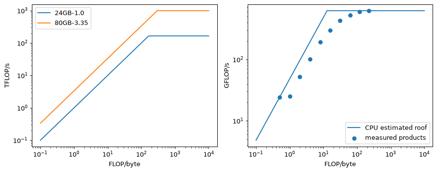
Interpretation. The two 24 GB profiles admit the same number of requests but have different decode speeds. On the CPU, aggregate arithmetic throughput usually rises with B even though individual products become slower. A roofline identifies a possible bottleneck; points can lie far below it because of overheads, locality and inefficient kernels.
Try next. Add a two-device profile with doubled capacity and bandwidth, then apply an assumed communication penalty. That estimate needs an interconnect model before it can guide a real purchase.
Lab 2 — A KV cache for a small decoder, and prefix caching by hand
Goal. Check cached logits against a full causal forward pass, measure exact cache bytes and expose position errors that token comparisons miss. The final step downloads about 270 MB of pinned SmolLM2-135M weights, reused by later labs. Everything runs on a CPU in float32 with four threads. Allow 35 minutes.
Build an untrained decoder with explicit positions
Random weights are sufficient: cache correctness is an algebraic property, not a language-learning result. The model has four blocks, width 256, eight query heads, two KV heads and a 688-wide SwiGLU intermediate. Caches remain in their compact two-head representation; repetition happens only for attention.
import copy
import time
import statistics
import torch
from torch import nn
import torch.nn.functional as F
from transformers import AutoTokenizer, AutoModelForCausalLM, DynamicCache

torch.set_num_threads(4)
torch.manual_seed(0)

class RMS(nn.Module):
    def __init__(self,d):
        super().__init__(); self.weight=nn.Parameter(torch.ones(d))
    def forward(self,x):
        return x*torch.rsqrt(x.square().mean(-1,keepdim=True)+1e-5)*self.weight

def rope(x,start):
    # Split-half RoPE; positions are absolute, including a reused prefix.
    half=x.shape[-1]//2
    freq=10000.**(-torch.arange(half,dtype=x.dtype)/half)
    angles=torch.arange(start,start+x.shape[-2],dtype=x.dtype)[:,None]*freq[None,:]
    c=angles.cos()[None,None]; s=angles.sin()[None,None]
    a,b=x[...,:half],x[...,half:]
    return torch.cat((a*c-b*s,a*s+b*c),dim=-1)

class Block(nn.Module):
    def __init__(self):
        super().__init__()
        self.n1=RMS(256); self.n2=RMS(256)
        self.q=nn.Linear(256,256,bias=False)
        self.k=nn.Linear(256,64,bias=False); self.v=nn.Linear(256,64,bias=False)
        self.o=nn.Linear(256,256,bias=False)
        self.gate=nn.Linear(256,688,bias=False)
        self.up=nn.Linear(256,688,bias=False); self.down=nn.Linear(688,256,bias=False)
    def forward(self,x,past,start):
        z=self.n1(x); b,t,_=z.shape
        q=rope(self.q(z).view(b,t,8,32).transpose(1,2),start)
        k=rope(self.k(z).view(b,t,2,32).transpose(1,2),start)
        v=self.v(z).view(b,t,2,32).transpose(1,2)
        old=0 if past is None else past[0].shape[2]
        if past is not None:
            k=torch.cat((past[0],k),2); v=torch.cat((past[1],v),2)
        mask=torch.arange(k.shape[2])[None,:] <= old+torch.arange(t)[:,None]
        a=F.scaled_dot_product_attention(q,k.repeat_interleave(4,1),v.repeat_interleave(4,1),attn_mask=mask)
        x=x+self.o(a.transpose(1,2).reshape(b,t,256))
        z=self.n2(x); x=x+self.down(F.silu(self.gate(z))*self.up(z))
        return x,(k,v)

class Decoder(nn.Module):
    def __init__(self):
        super().__init__(); self.emb=nn.Embedding(512,256)
        self.blocks=nn.ModuleList([Block() for _ in range(4)])
        self.norm=RMS(256); self.head=nn.Linear(256,512,bias=False)
    def forward(self,ids,past=None,start=0):
        x=self.emb(ids); cache=[]
        for i,block in enumerate(self.blocks):
            x,kv=block(x,None if past is None else past[i],start); cache.append(kv)
        return self.head(self.norm(x)),cache

toy=Decoder().eval()
prompt=torch.randint(0,512,(1,16),generator=torch.Generator().manual_seed(1))
print('Toy parameters:',sum(p.numel() for p in toy.parameters()))

@torch.inference_mode()
def generate(n,cached,bug=None):
    ids=prompt.clone(); cache=None; logs=[]
    for i in range(n):
        if not cached or i==0:
            logits,cache=toy(ids); last=logits[:,-1]
        else:
            pos=ids.shape[1]-1
            if bug=='off-by-one': pos-=1
            if bug=='frozen': pos=16
            logits,cache=toy(ids[:,-1:],cache,pos); last=logits[:,-1]
        logs.append(last.clone()); ids=torch.cat((ids,last.argmax(-1)[:,None]),1)
    return ids,torch.stack(logs),cache

reference,ref_logs,_=generate(256,False)
ids,logs,cache=generate(256,True)
measured=sum(k.numel()*k.element_size()+v.numel()*v.element_size() for k,v in cache)
t=cache[0][0].shape[2]
print('Tokens equal:',torch.equal(reference,ids),'max logit error: %.3g' % (logs-ref_logs).abs().max())
print('Cached tokens:',t,'measured bytes:',measured,'formula:',2*4*2*32*4*t)
for bug in ['off-by-one','frozen']:
    bad,badlogs,_=generate(256,True,bug)
    differences=(bad!=reference).nonzero()
    first=None if differences.numel()==0 else int(differences[0,1])-16
    print(bug,'tokens equal:',torch.equal(bad,reference),'first differing output:',first,
          'max logit error: %.3g' % (badlogs-ref_logs).abs().max())
print('n  uncached_s  cached_s')
for n in [64,128,256,512]:
    durations=[]
    for cached in [False,True]:
        begin=time.perf_counter(); generate(n,cached); durations.append(time.perf_counter()-begin)
    print(n, '%.3f %.3f' % tuple(durations))
Toy parameters: 3033344
Tokens equal: True max logit error: 1.79e-06
Cached tokens: 271 measured bytes: 555008 formula: 555008
off-by-one tokens equal: True first differing output: None max logit error: 0.0258
frozen tokens equal: False first differing output: 9 max logit error: 3.26
n  uncached_s  cached_s
64 0.120 0.055
128 0.332 0.110
256 0.974 0.243
512 3.241 0.491
The last emitted token has not yet been forwarded, so a 16-token prompt plus 256 emitted tokens leaves 271 cached positions. Compare logits only while both runs have the same prefix: after a bug changes a token, later differences include the changed context. The report above prints a whole-run diagnostic, not just the local error of the faulty rotation.
Reuse a real model’s prefix
Construct token sequences explicitly. Tokenising a prefix and suffix separately need not equal tokenising their concatenated strings: a boundary merge can change the final prefix token. Both paths below use the same concatenated ids, which is the condition needed for exact cache reuse. DynamicCache is mutable; copy it before branching to a new question. Do not override its inferred positions.
MODEL='HuggingFaceTB/SmolLM2-135M'
REV='93efa2f097d58c2a74874c7e644dbc9b0cee75a2'
tok=AutoTokenizer.from_pretrained(MODEL,revision=REV)
real=AutoModelForCausalLM.from_pretrained(MODEL,revision=REV,dtype=torch.float32,attn_implementation='sdpa').eval()
paragraph=('A safety case connects a claim about the pressure relief system to evidence. '
           'Separate assumptions, operating limits, faults, safeguards and remaining uncertainty. '
           'Each hazard log entry names the initiating event, consequence, prevention and evidence reference. '
           'A model drafts text for an engineer to check; it does not approve the system. ')
prefix=tok.encode(paragraph*60,add_special_tokens=False)[:3000]
questions=['\nExplain the evidence needed for a stuck valve.',
           '\nWhich assumptions should an engineer check?',
           '\nDraft a concise claim about overpressure protection.']
with torch.inference_mode():
    begin=time.perf_counter()
    shared=real(torch.tensor([prefix]),past_key_values=DynamicCache(config=real.config),use_cache=True).past_key_values
    initial=time.perf_counter()-begin
    print('Prefix tokens:',len(prefix),'one-time prefix seconds: %.3f' % initial)
    for question in questions:
        suffix=tok.encode(question,add_special_tokens=False)
        begin=time.perf_counter(); cold=real(torch.tensor([prefix+suffix]),use_cache=False).logits[:,-1]
        cold_s=time.perf_counter()-begin
        begin=time.perf_counter()
        warm=real(torch.tensor([suffix]),past_key_values=copy.deepcopy(shared),use_cache=True).logits[:,-1]
        warm_s=time.perf_counter()-begin
        error=(cold-warm).abs().max().item()
        assert torch.allclose(cold,warm,atol=2e-4,rtol=1e-5)
        print('suffix=%d cold=%.3fs warm=%.3fs max_error=%.3g' % (len(suffix),cold_s,warm_s,error))
Prefix tokens: 3000 one-time prefix seconds: 2.524
suffix=10 cold=2.511s warm=0.074s max_error=3.24e-05
suffix=8 cold=2.413s warm=0.063s max_error=2.48e-05
suffix=11 cold=2.453s warm=0.076s max_error=3.34e-05
Interpretation. The warm request avoids most prefix computation, while its new queries still attend to the prefix. It is not a shortcut through the model’s semantics. A position bug can survive a greedy-token test; the logit comparison is the stronger check.
Try next. Pre-allocate the toy cache to avoid repeated concatenation. Change the KV-head count and check the byte formula before timing anything.
Lab 3 — A continuous-batching simulator
Goal. Compare scheduling policies on an identical seeded workload, then find capacity under two latency objectives. This is an executable mathematical model, not a benchmark of any serving engine. Allow 30 minutes. No download is required.
Define the cost model and workload
The FLOP count includes each new position’s attention to its cached context. One hybrid iteration shares a weight read between prefill and decode: use the maximum of its memory and compute times, rather than adding them. This simplified model does not represent host overhead, page gathering or kernel-launch costs. It treats all cached positions as one contiguous pool; the on-demand policy models capacity, not a physical implementation of PagedAttention.
import math
import random
import heapq
from collections import deque
from dataclasses import dataclass, field
import numpy as np
import matplotlib.pyplot as plt

N=8927875072
L=36
D=4096
W=5.5e9

@dataclass
class Device:
    memory: float=16e9
    bandwidth: float=1e12
    compute: float=.5*165e12
    kv: int=147456

def iteration(decodes,chunks,device):
    # decodes: cached context lengths; chunks: (new tokens, cached tokens).
    positions=len(decodes)+sum(k for k,c in chunks)
    attention=sum(decodes)+sum(k*c+k*(k+1)/2 for k,c in chunks)
    flops=2*N*positions+4*L*D*attention
    moved=W+device.kv*(sum(decodes)+sum(c for k,c in chunks))
    return max(moved/device.bandwidth,flops/device.compute)

dev=Device()
print('prefill4000 %.3fs, decode18 %.2fms' % (iteration([],[(4000,0)],dev),1000*iteration([5000]*18,[],dev)))
for chunk in [512,128]:
    print('chunk',chunk,'17 decodes: %.2fms opening, %.2fms after2000' %
          (1000*iteration([5000]*17,[(chunk,0)],dev),1000*iteration([5000]*17,[(chunk,2000)],dev)))

@dataclass
class Request:
    arrival: float
    prompt: int
    output: int
    number: int
    filled: int=0
    generated: int=0
    stamps: list=field(default_factory=list)
    @property
    def context(self):
        return self.filled
    @property
    def required_prefill(self):
        return self.prompt+self.generated

def workload(rate,count=300):
    rng=random.Random(0); now=0.; requests=[]
    for number in range(count):
        now+=rng.expovariate(rate)
        prompt=rng.randint(2000,6000)
        output=min(4000,max(16,int(rng.lognormvariate(math.log(1500),.6))))
        requests.append(Request(now,prompt,output,number))
    return requests

sample=workload(.2)
print('Mean output %.1f, nominal .200, realised %.3f requests/s' %
      (np.mean([r.output for r in sample]),len(sample)/sample[-1].arrival))
prefill4000 0.923s, decode18 18.77ms
chunk 512 17 decodes: 116.04ms opening, 123.36ms after2000
chunk 128 17 decodes: 32.05ms opening, 33.88ms after2000
Mean output 1737.4, nominal .200, realised 0.224 requests/s
Run static and iteration-level policies
Static batches dispatch at 16 requests or after the oldest has waited two seconds. They retain padding slots until the longest output finishes. Static batches are not memory-checked: that favours them, since their worst-case cache can exceed the 16 GB budget. Continuous policies have a 256-sequence ceiling, first-in-first-out admission, either full-length reservations or actual-use admission. If growth exceeds memory, the newest running request is preempted and later re-prefills its original prompt and generated tokens. Chunking caps new prefill positions at 256 per iteration. Interrupted requests retain their previous token timestamps.
The first token is emitted at the end of prefill; each later token is emitted at the end of its decode iteration. There is no network delay in this model.
def metrics(requests,now,preemptions=0):
    ttft=np.array([r.stamps[0]-r.arrival for r in requests])
    gaps=np.concatenate([np.diff(r.stamps) for r in requests])
    e2e=np.array([r.stamps[-1]-r.arrival for r in requests])
    tpot=np.array([(r.stamps[-1]-r.stamps[0])/(r.output-1) for r in requests])
    good=sum((r.stamps[0]-r.arrival<=3 and max(np.diff(r.stamps))<=.1) for r in requests)
    return dict(ttft50=float(np.quantile(ttft,.5)),ttft99=float(np.quantile(ttft,.99)),
                itl50=float(np.quantile(gaps,.5)),itl99=float(np.quantile(gaps,.99)),itlmax=float(max(gaps)),
                tpot50=float(np.median(tpot)),e2e50=float(np.median(e2e)),
                throughput=sum(r.output for r in requests)/now,
                goodput=good/now,preemptions=preemptions,
                realised=len(requests)/requests[-1].arrival)

def simulate(rate,policy='chunked',device=None,count=300):
    device=Device() if device is None else device
    requests=workload(rate,count); pending=deque(requests)
    queue=deque(); running=[]; now=0.; completed=0; preemptions=0; iterations=0
    while completed<count:
        iterations+=1
        if iterations>2000000:
            raise RuntimeError('Simulation exceeded its bounded iteration budget')
        while pending and pending[0].arrival<=now:
            queue.append(pending.popleft())
        if not running and not queue:
            now=pending[0].arrival; continue
        if policy=='static':
            if not running:
                dispatch=queue[0].arrival+2
                if len(queue)<16 and now<dispatch:
                    now=min(dispatch,pending[0].arrival if pending else math.inf); continue
                running=[queue.popleft() for _ in range(min(16,len(queue)))]
                now+=iteration([],[(r.prompt,0) for r in running],device)
                for r in running:
                    r.filled=r.prompt; r.generated=1; r.stamps.append(now)
            else:
                now+=iteration([r.filled for r in running],[],device)
                for r in running:
                    r.filled+=1
                    if r.generated<r.output:
                        r.generated+=1; r.stamps.append(now)
                if all(r.generated==r.output for r in running):
                    completed+=len(running); running=[]
            continue
        # Reserve admission charges the full possible output. Actual admission
        # charges current cache plus the whole prompt of each new joiner.
        used=sum((r.prompt+4000 if policy=='reserve' else r.context)*device.kv for r in running)
        while queue and len(running)<256:
            r=queue[0]
            cost=(r.prompt+4000 if policy=='reserve' else r.required_prefill)*device.kv
            if used+cost>device.memory*.99: break
            queue.popleft(); running.append(r); used+=cost
        if not running:
            raise ValueError('A request cannot fit in the configured cache')
        budget=256 if policy=='chunked' else math.inf
        chunks=[]; decoding=[]; actions=[]
        for r in running:
            remaining=r.required_prefill-r.filled
            if remaining>0:
                k=int(min(remaining,budget))
                if k:
                    chunks.append((k,r.filled)); actions.append((r,k,True)); budget-=k
            else:
                decoding.append(r.filled); actions.append((r,1,False))
        growth=sum(k for r,k,is_prefill in actions)
        current=sum(r.context for r in running)
        if (current+growth)*device.kv>device.memory:
            victim=running.pop(); victim.filled=0; queue.appendleft(victim); preemptions+=1
            continue
        now+=iteration(decoding,chunks,device)
        for r,k,is_prefill in actions:
            r.filled+=k
            if not is_prefill or r.filled==r.required_prefill:
                r.generated+=1; r.stamps.append(now)
        finished=[r for r in running if r.generated==r.output]
        completed+=len(finished)
        running=[r for r in running if r.generated<r.output]
    return metrics(requests,now,preemptions)

rates=[.10,.20,.25,.30,.35,.40]
results={}
print('policy  nominal real  TTFTp50/p99s ITLp50/p99/maxms tok/s preempt')
for policy in ['static','reserve','paged','chunked']:
    results[policy]=[]
    for rate in rates:
        m=simulate(rate,policy); results[policy].append(m)
        print('%-7s %.2f %.3f %6.2f/%6.2f %5.1f/%5.1f/%7.1f %6.1f %5d' %
              (policy,rate,m['realised'],m['ttft50'],m['ttft99'],1000*m['itl50'],
               1000*m['itl99'],1000*m['itlmax'],m['throughput'],m['preemptions']))
fig,axes=plt.subplots(2,1,figsize=(7,6),sharex=True)
for policy,ms in results.items():
    axes[0].semilogy(rates,[m['ttft99'] for m in ms],label=policy+' p99')
    axes[0].semilogy(rates,[m['ttft50'] for m in ms],linestyle=':',alpha=.6)
    axes[1].semilogy(rates,[1000*m['itl99'] for m in ms],label=policy+' p99')
axes[0].axhline(3,color='black',linestyle='--'); axes[0].set_ylabel('TTFT seconds')
axes[1].axhline(100,color='black',linestyle='--'); axes[1].set(ylabel='ITL ms',xlabel='Nominal requests/s')
axes[0].legend(); fig.tight_layout(); plt.show()
policy  nominal real  TTFTp50/p99s ITLp50/p99/maxms tok/s preempt
static  0.10 0.112  13.04/ 52.59   7.9/ 14.5/   16.6  193.3     0
static  0.20 0.224 247.48/423.15  17.0/ 24.4/   25.3  295.0     0
static  0.25 0.281 385.93/710.34  17.0/ 24.1/   25.7  290.5     0
static  0.30 0.337 455.14/792.05  17.1/ 24.1/   25.7  302.7     0
static  0.35 0.393 507.56/940.23  17.2/ 24.3/   25.3  301.2     0
static  0.40 0.449 551.91/1035.02  17.2/ 24.3/   25.3  301.3     0
reserve 0.10 0.112   1.01/  2.65   7.3/ 12.8/ 2337.9  193.6     0
reserve 0.20 0.224   1.10/  6.53  10.2/ 16.2/ 2338.2  384.2     0
reserve 0.25 0.281   1.29/ 21.52  14.2/ 16.8/ 3130.1  477.7     0
reserve 0.30 0.337  45.34/ 73.68  15.3/ 17.2/ 2194.9  548.4     0
reserve 0.35 0.393 114.24/170.96  15.3/ 17.2/ 2576.3  553.9     0
reserve 0.40 0.449 159.43/251.51  15.3/ 17.2/ 2576.3  556.9     0
paged   0.10 0.112   1.01/  2.65   7.3/ 12.8/ 2337.9  193.6     0
paged   0.20 0.224   1.08/  2.94  10.2/ 17.6/ 2338.2  384.2     0
paged   0.25 0.281   1.14/  3.52  13.8/ 21.4/ 3130.1  477.7     2
paged   0.30 0.337  20.56/ 46.29  21.0/ 21.5/15405.2  564.0    46
paged   0.35 0.393  86.34/136.90  21.1/ 21.5/10245.8  571.1    52
paged   0.40 0.449 142.72/234.65  21.1/ 21.5/15395.6  564.8    64
chunked 0.10 0.112   1.01/  2.20   7.3/ 58.0/   65.9  193.6     0
chunked 0.20 0.224   1.09/  2.89  10.1/ 61.6/   65.9  384.3     0
chunked 0.25 0.281   1.15/  3.07  12.9/ 62.6/   66.0  477.9     0
chunked 0.30 0.337   1.53/ 29.87  19.4/ 63.9/ 6433.1  570.3   280
chunked 0.35 0.393  74.71/116.71  21.2/ 64.3/10303.5  586.9  1966
chunked 0.40 0.449 122.92/201.47  21.3/ 64.3/10131.6  589.2  2694
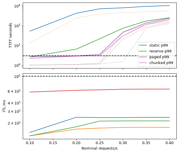
Find an operating point, then price its measured throughput
The bisection assumes pass/fail is locally monotonic. Check nearby rates before using a result: finite sampled percentiles and scheduler transitions can violate that assumption. Both objectives are pooled percentile objectives; they do not mean that every request meets a maximum-gap bound. The separately printed goodput uses a stricter per-request maximum-gap rule.
def capacity(device):
    low,high=.01,4.
    for _ in range(10):
        mid=(low+high)/2
        m=simulate(mid,'chunked',device)
        if m['ttft99']<=3 and m['itl99']<=.1: low=mid
        else: high=mid
    m=simulate(low,'chunked',device)
    return low,m

profiles=[('24GB-bf16',Device(),1.),('24GB-int8',Device(kv=73728),1.),
          ('H100-bf16',Device(memory=72e9,bandwidth=3.35e12,compute=.5*989e12),2.5),
          ('L4-bf16',Device(bandwidth=.30e12,compute=.5*121e12),.8)]
print('Prices below are assumptions, not current quotes.')
for name,device,price in profiles:
    rate,m=capacity(device)
    cost=price*1e6/(3600*m['throughput'])
    nearby=[simulate(rate+delta,'chunked',device) for delta in [-.005,.005]]
    passes=[v['ttft99']<=3 and v['itl99']<=.1 for v in nearby]
    print('%s nominal=%.3f/s realised=%.3f/s nominal_requests/h=%.0f output=%.1f tok/s USD/million=%.3f goodput=%.3f/s nearby_pass=%s' %
          (name,rate,m['realised'],rate*3600,m['throughput'],cost,m['goodput'],passes))
Prices below are assumptions, not current quotes.
24GB-bf16 nominal=0.244/s realised=0.274/s nominal_requests/h=878 output=466.3 tok/s USD/million=0.596 goodput=0.266/s nearby_pass=[True, False]
24GB-int8 nominal=0.252/s realised=0.282/s nominal_requests/h=906 output=482.1 tok/s USD/million=0.576 goodput=0.275/s nearby_pass=[True, False]
H100-bf16 nominal=2.196/s realised=2.464/s nominal_requests/h=7905 output=3500.0 tok/s USD/million=0.198 goodput=2.008/s nearby_pass=[True, False]
L4-bf16 nominal=0.065/s realised=0.072/s nominal_requests/h=232 output=124.0 tok/s USD/million=1.792 goodput=0.071/s nearby_pass=[True, False]
Interpretation. Increasing load improves batching until queueing or cache pressure takes over. Chunking trades a few longer decode iterations for removal of whole-prompt stalls. An 8-bit cache changes capacity and traffic simultaneously; this simulation assumes its quality and scale overhead are acceptable, which a deployment must test. Cost comes from the printed output tokens per second, not from nominal arrivals multiplied by an invented output length.
Try next. Make static batches memory-aware. Add bursty arrivals or a small share of long documents and repeat the SLO search. Record the changed assumptions alongside every result.
Lab 4 — Quantisation from scratch: weights, outliers and activations
Goal. Measure the error caused by quantisation and separate weight error from
activation error. Allow 40 minutes. The first run downloads pinned SmolLM2-135M
weights (about 270 MB, already cached after Lab 2) and a 0.73 MB WikiText-2 test
parquet file. Install pandas and pyarrow alongside PyTorch and Transformers.
Use float32 CPU inference, four threads and QUICK = True for four evaluation
windows; the displayed full run uses eight. Calibration and evaluation windows
are disjoint, although both come from the same dataset.
Load the model and fixed text windows
import math
import torch
import numpy as np
import pandas as pd
import matplotlib.pyplot as plt
from torch import nn
import torch.nn.functional as F
from transformers import AutoTokenizer, AutoModelForCausalLM
from huggingface_hub import hf_hub_download

torch.set_num_threads(4)
torch.manual_seed(0)
QUICK=False
MODEL='HuggingFaceTB/SmolLM2-135M'
REV='93efa2f097d58c2a74874c7e644dbc9b0cee75a2'
DATA_REV='b08601e04326c79dfdd32d625aee71d232d685c3'
tok=AutoTokenizer.from_pretrained(MODEL,revision=REV)
model=AutoModelForCausalLM.from_pretrained(MODEL,revision=REV,dtype=torch.float32,attn_implementation='sdpa').eval()
path=hf_hub_download('Salesforce/wikitext','wikitext-2-raw-v1/test-00000-of-00001.parquet',
                     repo_type='dataset',revision=DATA_REV)
text='\n\n'.join(pd.read_parquet(path)['text'].tolist())
ids=torch.tensor(tok.encode(text,add_special_tokens=False))
windows=4 if QUICK else 8
evaluation=ids[:windows*512].reshape(windows,512)
calibration=ids[200000:200000+4*512].reshape(4,512)
linears={name:layer for name,layer in model.named_modules()
         if isinstance(layer,nn.Linear) and name!='lm_head'}
original={name:layer.weight.detach().clone() for name,layer in linears.items()}
print('Text tokens:',len(ids),'evaluation tokens:',evaluation.numel())
print('Linear layers:',len(linears),'quantised parameters:',sum(w.numel() for w in original.values()))

@torch.inference_mode()
def perplexity():
    total=0.; count=0
    for batch in evaluation.split(4):
        logits=model(batch,use_cache=False).logits[:,:-1]
        labels=batch[:,1:]
        total+=F.cross_entropy(logits.reshape(-1,logits.shape[-1]),labels.reshape(-1),reduction='sum').item()
        count+=labels.numel()
    return math.exp(total/count)

baseline=perplexity()
print('float32 perplexity: %.4f' % baseline)
Text tokens: 304986 evaluation tokens: 4096
Linear layers: 210 quantised parameters: 106168320
float32 perplexity: 20.8462
Windows have 511 scored next-token predictions each; cross-window predictions are excluded. Perplexity is the exponential of their mean loss. It is not the mean of window perplexities. Tokenisation, joining convention and window boundaries all matter when comparing this result with a paper.
Quantise and immediately dequantise
This is fake quantisation: it simulates rounding damage but leaves float32 tensors and kernels in place. The printed storage is a hypothetical packed size of the linear layers, excluding embeddings, norms, headers and alignment. It is not the process memory and it predicts no speed-up in this lab.
def quantise(w,bits=8,mode='tensor',zero=False,group=64):
    shape=w.shape
    if mode=='tensor': rows=w.reshape(1,-1)
    elif mode=='channel': rows=w.reshape(w.shape[0],-1)
    elif mode=='group': rows=w.reshape(-1,group)
    else: raise ValueError(mode)
    if zero:
        lo=rows.amin(-1,keepdim=True); hi=rows.amax(-1,keepdim=True)
        scale=((hi-lo)/(2**bits-1)).clamp_min(1e-12)
        zp=torch.round(-lo/scale)
        q=(torch.round(rows/scale)+zp).clamp(0,2**bits-1)
        out=scale*(q-zp)
    else:
        top=2**(bits-1)-1
        scale=(rows.abs().amax(-1,keepdim=True)/top).clamp_min(1e-12)
        out=torch.round(rows/scale).clamp(-top,top)*scale
    return out.reshape(shape)

def restore():
    with torch.no_grad():
        for name,layer in linears.items(): layer.weight.copy_(original[name])

records=[]
schemes=[('int8 tensor',8,'tensor',False),('int8 channel',8,'channel',False),
         ('int4 tensor',4,'tensor',False),('int4 channel',4,'channel',False),
         ('int4 group64',4,'group',False),('int4 group64 zero',4,'group',True)]
print('scheme              bits/w  linearMB mean_rel_error perplexity')
for label,bits,mode,zero in schemes:
    errors=[]; storage=0.
    with torch.no_grad():
        for name,layer in linears.items():
            w=original[name]; qw=quantise(w,bits,mode,zero)
            layer.weight.copy_(qw); errors.append(((w-qw).norm()/w.norm()).item())
            groups=1 if mode=='tensor' else (w.shape[0] if mode=='channel' else w.numel()//64)
            storage+=w.numel()*bits/8 + groups*(4 if zero else 2)
    n=sum(w.numel() for w in original.values())
    bpw=storage*8/n; ppl=perplexity()
    records.append((label,bpw,ppl))
    print('%-19s %6.3f %8.2f %14.4f %10.4f' % (label,bpw,storage/1e6,np.mean(errors),ppl))
restore()
scheme              bits/w  linearMB mean_rel_error perplexity
int8 tensor          8.000   106.17         0.0290    21.6252
int8 channel         8.023   106.48         0.0085    20.9937
int4 tensor          4.000    53.08         0.4889 5834512.4874
int4 channel         4.023    53.40         0.1546    46.2519
int4 group64         4.250    56.40         0.1136    29.1763
int4 group64 zero    4.500    59.72         0.0947    27.1402
Find activation outliers on calibration text
Hooks see the input to each linear layer. Per-input-channel maxima are pooled over all calibration tokens, then compared with the median channel. The worst weight ratio uses the same input-channel orientation. No evaluation activations select the smoothing scales.
stats={}; hooks=[]
for name,layer in linears.items():
    def collect(module,args,name=name):
        x=args[0].detach().reshape(-1,args[0].shape[-1]).abs().amax(0)
        stats[name]=x if name not in stats else torch.maximum(stats[name],x)
    hooks.append(layer.register_forward_pre_hook(collect))
with torch.inference_mode():
    for batch in calibration.split(2): model(batch,use_cache=False)
for hook in hooks: hook.remove()
ratios={name:float(x.max()/x.median().clamp_min(1e-12)) for name,x in stats.items()}
worst=max(ratios,key=ratios.get)
weight_ratios=[]
for w in original.values():
    x=w.abs().amax(0); weight_ratios.append(float(x.max()/x.median()))
print('Worst activation layer:',worst)
print('max=%.3f median=%.3f ratio=%.1f' % (stats[worst].max(),stats[worst].median(),ratios[worst]))
print('Median activation ratio %.2f; worst weight ratio %.2f' % (np.median(list(ratios.values())),max(weight_ratios)))
Worst activation layer: model.layers.11.mlp.down_proj
max=2479.243 median=1.307 ratio=1897.2
Median activation ratio 7.95; worst weight ratio 12.42
Simulate W8A8 and SmoothQuant
For PyTorch’s row-oriented weight matrix the equivalent transformation is
weight * s and input / s. Hooks apply the division explicitly so its effect
is visible; this code does not implement fused production kernels. Folding scales
into preceding operations requires respecting every consumer of the activation;
some projections need more care than changing one RMSNorm vector.
for alpha in [None,.5,.8]:
    restore(); hooks=[]
    with torch.no_grad():
        for name,layer in linears.items():
            w=original[name]
            s=torch.ones(w.shape[1]) if alpha is None else (
                stats[name].clamp_min(1e-8)**alpha /
                w.abs().amax(0).clamp_min(1e-8)**(1-alpha))
            layer.weight.copy_(quantise(w*s,8,'channel'))
            def activation(module,args,s=s):
                return (quantise(args[0]/s,8,'tensor'),)
            hooks.append(layer.register_forward_pre_hook(activation))
    ppl=perplexity()
    label='W8A8' if alpha is None else 'SmoothQuant %.1f' % alpha
    print(label,'perplexity %.4f' % ppl); records.append((label,8.03,ppl))
    for hook in hooks: hook.remove()
restore()
fig,ax=plt.subplots(figsize=(8,4))
for i,(label,bits,ppl) in enumerate(records):
    ax.scatter(bits,ppl); ax.annotate(label,(bits,ppl),xytext=(5,4+i%3*10),textcoords='offset points',fontsize=8)
ax.axhline(baseline,linestyle='--',color='black',label='float32 baseline')
ax.set(yscale='log',xlabel='Bits per stored linear weight',ylabel='Perplexity'); ax.legend()
fig.tight_layout(); plt.show()
W8A8 perplexity 40.8337
SmoothQuant 0.5 perplexity 26.2966
SmoothQuant 0.8 perplexity 23.6349
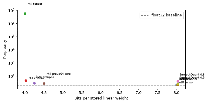
Interpretation. Finer weight granularity usually helps, but activation outliers can spoil otherwise accurate int8 weights. SmoothQuant redistributes range before rounding. It preserves the unquantised product, not the rounded product. These results concern a 135M model, one short text sample and these simple quantisers; they do not establish a universal quality loss for int4 or calibrated methods.
Try next. Leave the down-projections at eight bits and measure the trade-off. Use a held-out engineering task as well as generic perplexity before promoting any quantised artifact.
Lab 5 — Speculative decoding from scratch
Goal. Preserve a target model’s greedy output while proposing several tokens at once, then verify the stochastic acceptance theorem separately. Allow 35 minutes. This downloads about 724 MB for pinned SmolLM2-360M, plus the 270 MB draft already used by Lab 2. Both run in float32 on a CPU. A CPU gain is an experimental result, not a requirement for the algorithm to be correct.
Load compatible models and measure step costs
The vocabulary ids must mean the same tokens. We check the complete tokenizer mapping, not only vocabulary size. Warm up before timing and use medians. The timed short-context steps are an approximation to the later generation costs.
import math
import time
import statistics
import torch
from transformers import AutoTokenizer, AutoModelForCausalLM, DynamicCache

torch.set_num_threads(4)
torch.manual_seed(0)
DRAFT='HuggingFaceTB/SmolLM2-135M'
TARGET='HuggingFaceTB/SmolLM2-360M'
DREV='93efa2f097d58c2a74874c7e644dbc9b0cee75a2'
TREV='f8027fd0eaeea54caa13c31d31b9fdc459c38b49'
tok=AutoTokenizer.from_pretrained(DRAFT,revision=DREV)
target_tok=AutoTokenizer.from_pretrained(TARGET,revision=TREV)
assert tok.get_vocab()==target_tok.get_vocab()
draft=AutoModelForCausalLM.from_pretrained(DRAFT,revision=DREV,dtype=torch.float32,attn_implementation='sdpa').eval()
target=AutoModelForCausalLM.from_pretrained(TARGET,revision=TREV,dtype=torch.float32,attn_implementation='sdpa').eval()
print('Draft parameters:',sum(p.numel() for p in draft.parameters()))
print('Target parameters:',sum(p.numel() for p in target.parameters()))

@torch.inference_mode()
def step_cost(model,width):
    prefix=torch.tensor([tok.encode('A safety case links a claim to evidence and states assumptions about the system.',add_special_tokens=False)])
    cache=model(prefix,past_key_values=DynamicCache(config=model.config),use_cache=True).past_key_values
    length=cache.get_seq_length(); suffix=torch.full((1,width),100,dtype=torch.long)
    durations=[]
    for i in range(23):
        cache.crop(length)
        begin=time.perf_counter(); model(suffix,past_key_values=cache,use_cache=True)
        elapsed=time.perf_counter()-begin
        if i>=3: durations.append(elapsed)
    return statistics.median(durations)

td=step_cost(draft,1); tt=step_cost(target,1)
verification={g:step_cost(target,g+1)/tt for g in [2,4,6]}
c=td/tt
print('Draft %.2fms target %.2fms c=%.3f' % (td*1000,tt*1000,c))
for g,v in verification.items(): print('gamma=%d verification=%.3f target steps' % (g,v))
Draft parameters: 134515008
Target parameters: 361821120
Draft 17.02ms target 38.07ms c=0.447
gamma=2 verification=1.188 target steps
gamma=4 verification=1.224 target steps
gamma=6 verification=1.281 target steps
Implement the target baseline and cache rollback
At an iteration boundary the target cache covers all committed tokens except the last. The target scores that last token and all proposals together, producing predictions for the proposals and one bonus. After rejection, crop away all uncommitted states. The draft may lag by one accepted token; its next call feeds every committed token missing from its cache. This avoids silently giving the draft the wrong prefix after a fully accepted iteration.
@torch.inference_mode()
def greedy(model,ids,n=64):
    out=ids.clone(); cache=DynamicCache(config=model.config)
    if ids.shape[1]>1: model(ids[:,:-1],past_key_values=cache,use_cache=True)
    for _ in range(n):
        logits=model(out[:,cache.get_seq_length():],past_key_values=cache,use_cache=True).logits[:,-1]
        out=torch.cat((out,logits.argmax(-1)[:,None]),1)
    return out

@torch.inference_mode()
def speculative(ids,n=64,gamma=4):
    out=ids.clone(); initial=out.shape[1]
    dc=DynamicCache(config=draft.config); tc=DynamicCache(config=target.config)
    if initial>1:
        draft(out[:,:-1],past_key_values=dc,use_cache=True)
        target(out[:,:-1],past_key_values=tc,use_cache=True)
    accepted=0; rejected=0; iterations=0; min_gap=math.inf
    while out.shape[1]<initial+n:
        base=out.shape[1]; proposed=out.clone()
        for _ in range(gamma):
            logits=draft(proposed[:,dc.get_seq_length():],past_key_values=dc,use_cache=True).logits[:,-1]
            proposed=torch.cat((proposed,logits.argmax(-1)[:,None]),1)
        scores=target(proposed[:,tc.get_seq_length():],past_key_values=tc,use_cache=True).logits[0]
        picks=scores.argmax(-1); proposals=proposed[0,base:]
        k=0
        while k<gamma and proposals[k]==picks[k]: k+=1
        accepted+=k; rejected+=int(k<gamma); iterations+=1
        gaps=scores.topk(2,dim=-1).values
        min_gap=min(min_gap,float((gaps[:,0]-gaps[:,1]).min()))
        emitted=torch.cat((proposals[:k],picks[k:k+1]))
        remaining=initial+n-base
        out=torch.cat((out,emitted[:remaining][None]),1)
        committed=out.shape[1]-1
        tc.crop(committed); dc.crop(min(committed,dc.get_seq_length()))
    return out,accepted,rejected,iterations,min_gap

prompts=['A safety case is a structured argument that',
         'The main steps of a hazard analysis and risk assessment are',
         'def fibonacci(n):\n    ',
         'The industrial revolution began in',
         'Thermal runaway in a lithium-ion battery occurs when']
inputs=[torch.tensor([tok.encode(p,add_special_tokens=False)]) for p in prompts]
_ = greedy(target,inputs[0],4)
begin=time.perf_counter(); baseline=[greedy(target,x) for x in inputs]
baseline_s=time.perf_counter()-begin
print('Target baseline %.3fs, %.2f output tok/s' % (baseline_s,320/baseline_s))
for gamma in [2,4,6]:
    begin=time.perf_counter(); runs=[speculative(x,gamma=gamma) for x in inputs]
    elapsed=time.perf_counter()-begin
    a=sum(r[1] for r in runs); rejects=sum(r[2] for r in runs); iters=sum(r[3] for r in runs)
    alpha=a/(a+rejects); expected=sum(alpha**k for k in range(gamma+1))
    matches=[torch.equal(r[0],b) for r,b in zip(runs,baseline)]
    print('gamma=%d alpha=%.3f tokens/iter=%.3f predicted=%.3f equal=%s time=%.3fs speedup=%.3f predicted_speedup=%.3f min_verified_gap=%.3g' %
          (gamma,alpha,320/iters,expected,matches,elapsed,baseline_s/elapsed,
           expected/(gamma*c+verification[gamma]),min(r[4] for r in runs)))
    assert all(matches), 'Inspect the first differing token and its target top-two gap'
Target baseline 12.442s, 25.72 output tok/s
gamma=2 alpha=0.850 tokens/iter=2.540 predicted=2.574 equal=[True, True, True, True, True] time=11.146s speedup=1.116 predicted_speedup=1.236 min_verified_gap=0.00274
gamma=4 alpha=0.865 tokens/iter=3.636 predicted=3.819 equal=[True, True, True, True, True] time=11.082s speedup=1.123 predicted_speedup=1.268 min_verified_gap=0.00273
gamma=6 alpha=0.864 tokens/iter=4.324 predicted=4.711 equal=[True, True, True, True, True] time=12.294s speedup=1.012 predicted_speedup=1.189 min_verified_gap=0.00274
The final iteration is truncated at 64 output tokens. Its discarded proposals still cost time, so measured tokens per iteration can lie below the untruncated geometric prediction. Acceptance events also need not be independent. A mismatch would require diagnosis: either rollback/indexing is wrong or different numerical kernels changed a near-tied argmax. It is not evidence that stochastic speculation should intentionally alter the target distribution.
Check stochastic exactness without generating 200,000 sentences
One conditional next-token distribution is enough to test the acceptance identity. The vectorised trial below samples from the full 49,152-token vocabulary. Finite-sample total variation is positive, even for a correct algorithm.
with torch.inference_mode():
    ids=inputs[1]
    p=target(ids,use_cache=False).logits[0,-1].softmax(-1)
    q=draft(ids,use_cache=False).logits[0,-1].softmax(-1)
    overlap=torch.minimum(p,q).sum()
    residual=(p-q).clamp_min(0); residual/=residual.sum()
    count=200000
    torch.manual_seed(0)
    candidates=torch.multinomial(q,count,replacement=True)
    accept=torch.rand(count)<(p[candidates]/q[candidates]).clamp(max=1)
    replacements=torch.multinomial(residual,count,replacement=True)
    emitted=torch.where(accept,candidates,replacements)
    empirical=torch.bincount(emitted,minlength=p.numel()).float()/count
    analytic=torch.minimum(p,q)+(1-overlap)*residual
    print('Acceptance empirical %.5f analytic %.5f' % (accept.float().mean(),overlap))
    print('TV(empirical,p)=%.5f TV(q,p)=%.5f analytic_max_error=%.3g' %
          (.5*(empirical-p).abs().sum(),.5*(q-p).abs().sum(),(analytic-p).abs().max()))
    for token in p.topk(5).indices:
        print(repr(tok.decode([int(token)])),'p=%.5f empirical=%.5f' % (p[token],empirical[token]))
Acceptance empirical 0.80998 analytic 0.81007
TV(empirical,p)=0.01633 TV(q,p)=0.18995 analytic_max_error=4.42e-06
':' p=0.36838 empirical=0.36836
' as' p=0.17046 empirical=0.17063
' to' p=0.06203 empirical=0.06236
' listed' p=0.05193 empirical=0.05187
' described' p=0.04327 empirical=0.04262
Interpretation. Correctness and acceleration are separate questions. The acceptance/residual identity restores the target probabilities. Acceleration depends on acceptance, draft cost, verification cost and load. These two small CPU models are useful for inspection, even if the speed-up is modest or negative.
Try next. Replace the neural draft with a matching n-gram continuation from the prompt on a copying task. Keep target verification and rollback unchanged.
Lab 6 — Batched generation on a CPU: throughput and determinism
Goal. Measure what batching does to throughput and to each request’s speed, then compare one prompt alone and in a batch. Allow 20 minutes. Use the pinned SmolLM2-135M weights already cached in Lab 2; no server or new download is needed. This is a fixed-batch CPU experiment, not an open-loop serving load test.
Left-pad prompts and supply the correct positions
Left padding makes each row’s last input column a real token. The position ids come from its attention mask, so padding does not move its real tokens along the RoPE positions. Cached tensor length still includes padded columns: physical cache length and a row’s semantic position are different quantities.
import time
import statistics
import torch
import numpy as np
import matplotlib.pyplot as plt
from transformers import AutoTokenizer, AutoModelForCausalLM, DynamicCache

torch.set_num_threads(4)
torch.manual_seed(0)
MODEL='HuggingFaceTB/SmolLM2-135M'
REV='93efa2f097d58c2a74874c7e644dbc9b0cee75a2'
tok=AutoTokenizer.from_pretrained(MODEL,revision=REV)
tok.pad_token=tok.eos_token; tok.padding_side='left'
model=AutoModelForCausalLM.from_pretrained(MODEL,revision=REV,dtype=torch.float32,attn_implementation='sdpa').eval()
prompts=['The pressure relief valve protects the reactor vessel from overpressure.',
         'A hazard log entry identifies an initiating event, a consequence and the evidence for each credited safeguard.',
         'An engineer checks every assumption in the safety case before accepting a claim.',
         'The reactor vessel pressure sensor should detect a dangerous rise in pressure.',
         'A blocked discharge pipe changes the performance of the relief system because',
         'Evidence for the inspection interval includes operating records and the results of a component test.',
         'A claim without an evidence reference should be marked for review.',
         'The model drafts a structured argument, while a competent engineer checks its validity against the plant design.',
         'The industrial revolution began in Britain and spread because',
         'The first step in debugging a Python program is to reproduce the error.',
         'A function that sorts a list of integers returns',
         'A normal distribution is described by its mean and variance.',
         'The Earth orbits the Sun once every year because',
         'A robust measurement records its units and uncertainty.',
         'The operator follows the shutdown procedure when the pressure exceeds its allowed operating limit.',
         'A test of the backup protection system should include the failure of its primary sensor.']
print('Parameters:',sum(p.numel() for p in model.parameters()))
print('Prompt lengths:',[len(tok.encode(p,add_special_tokens=False)) for p in prompts])

@torch.inference_mode()
def batched_greedy(texts,n_new=64,keep_logits=False):
    encoded=tok(texts,return_tensors='pt',padding=True,add_special_tokens=False)
    ids=encoded.input_ids; mask=encoded.attention_mask
    pos=(mask.cumsum(-1)-1).clamp_min(0)
    next_pos=pos[:,-1:]+1
    cache=DynamicCache(config=model.config)
    begin=time.perf_counter()
    result=model(ids,attention_mask=mask,position_ids=pos,past_key_values=cache,use_cache=True)
    prefill=time.perf_counter()-begin
    logits=result.logits[:,-1]; logs=[logits[0].clone()] if keep_logits else []
    tokens=[logits.argmax(-1)]; times=[]
    for _ in range(n_new-1):
        mask=torch.cat((mask,torch.ones_like(mask[:,:1])),1)
        begin=time.perf_counter()
        result=model(tokens[-1][:,None],attention_mask=mask,position_ids=next_pos,
                     past_key_values=cache,use_cache=True)
        times.append(time.perf_counter()-begin)
        next_pos+=1; logits=result.logits[:,-1]; tokens.append(logits.argmax(-1))
        if keep_logits: logs.append(logits[0].clone())
    return torch.stack(tokens,1),prefill,times,(torch.stack(logs) if keep_logits else None),ids.shape[1]

# Replace these with your own Lab 1 measurements.
CPU_BW_GB=48.24
CPU_PEAK_GFLOPS=621.6
n=sum(p.numel() for p in model.parameters())
rows=[]
print('B TTFTms stepms per_sequence aggregate predictedms measured/predicted')
for b in [1,2,4,8,16]:
    batched_greedy(prompts[:b],4)
    tokens,ttft,times,_,padded=batched_greedy(prompts[:b])
    sec=statistics.median(times); ctx=padded+32
    memory=(4*n+b*46080*ctx)/(CPU_BW_GB*1e9)
    compute=(2*n*b+4*30*576*ctx*b)/(CPU_PEAK_GFLOPS*1e9)
    predicted=max(memory,compute)
    rows.append((b,1/sec,b/sec,1/predicted,b/predicted))
    print('%2d %7.2f %6.2f %12.2f %9.2f %11.2f %18.2f' %
          (b,ttft*1000,sec*1000,1/sec,b/sec,predicted*1000,sec/predicted))
fig,ax=plt.subplots(figsize=(7,4))
for column,label in [(1,'per sequence'),(2,'aggregate')]:
    ax.plot([r[0] for r in rows],[r[column] for r in rows],'o-',label=label)
    ax.plot([r[0] for r in rows],[r[column+2] for r in rows],'--',label=label+' roofline')
ax.set(xscale='log',yscale='log',xlabel='Batch size',ylabel='Output tokens/s'); ax.legend()
fig.tight_layout(); plt.show()
Parameters: 134515008
Prompt lengths: [12, 19, 14, 13, 12, 16, 12, 19, 9, 14, 9, 11, 9, 9, 15, 16]
B TTFTms stepms per_sequence aggregate predictedms measured/predicted
 1   39.39  17.69        56.54     56.54       11.20               1.58
 2   36.37  21.80        45.87     91.74       11.25               1.94
 4   57.29  22.86        43.74    174.97       11.35               2.01
 8  121.52  26.39        37.90    303.16       11.54               2.29
16  161.47  30.59        32.69    523.05       11.93               2.56
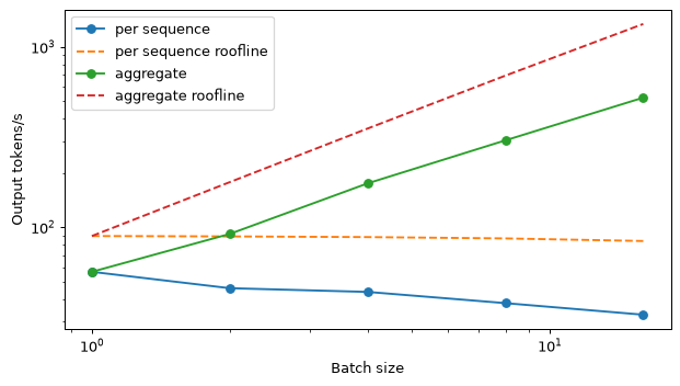
The measured prefill interval includes only the model forward, while a client’s TTFT includes tokenisation, scheduling, sampling and transport too. Per-sequence tokens/s here uses the median decode step; aggregate tokens/s multiplies that by B. Neither is an end-to-end service capacity. The model keeps generating for 64 positions even after an EOS, so comparisons have identical lengths.
Compare the same semantic prompt across batch shapes
solo,_,_,solo_logits,_=batched_greedy(prompts[:1],keep_logits=True)
batch,_,_,batch_logits,padded=batched_greedy(prompts[:8],keep_logits=True)
diff=(solo_logits-batch_logits).abs().amax(-1)
top=solo_logits.topk(2,dim=-1).values
gaps=top[:,0]-top[:,1]; smallest=int(gaps.argmin())
same=torch.equal(solo[0],batch[0]); differences=(solo[0]!=batch[0]).nonzero()
first=None if differences.numel()==0 else int(differences[0])
print('Padding columns for row0:',padded-len(tok.encode(prompts[0],add_special_tokens=False)))
print('Tokens equal:',same,'first differing output:',first)
print('Max logit difference %.6g; median %.6g' % (diff.max(),diff.median()))
print('Smallest top-two gap %.6g at output step %d' % (gaps[smallest],smallest))
if not same:
    print('Gap at first difference:',float(gaps[first]))
Padding columns for row0: 7
Tokens equal: True first differing output: None
Max logit difference 5.76973e-05; median 3.52859e-05
Smallest top-two gap 0.0557842 at output step 22
If the outputs diverge, logit comparisons after the first differing token mix arithmetic differences with different conditioning text. Inspect the first difference on a common prefix. Identical outputs on this finite test support that particular run; they do not guarantee equality under another precision or engine.
Try next. Extend the output to 512 tokens, compare different padding lengths and record the first differing token. An optional GPU extension is to serve a supported small model with vLLM and repeat with streamed client timestamps and open-loop arrivals; engine installation, GPU memory and downloads are additional requirements, so no main-text result depends on that extension.
Exercises
Work the estimates from their assumptions before opening the solutions. The 15 exercises take about 130 minutes: seven introductory, seven intermediate and one capacity-planning project. Decimal units apply unless a binary unit is explicitly named. Hardware ceilings and assumed prices are not measured service performance or current quotes.
A colleague estimates batch-one decode for a 9B bf16 model on a 989 TFLOP/s, 3.35 TB/s device as 989\times10^{12}/(2\times9\times10^9)\approx55{,}000 tokens/s. What is wrong, and what is the correct order of magnitude?
Show solution
The division gives an arithmetic ceiling while ignoring weight traffic. Batch-one bf16 projections have intensity near one FLOP/byte, far below the device’s 989/3.35\approx295 ridge. Reading roughly 18 GB per token takes 18\times10^9/(3.35\times10^{12})\approx0.00537 s, or about 186 tokens/s. Cache reads, incomplete bandwidth use and overhead lower the achievable rate. The order is hundreds, not tens of thousands, of tokens/s. A compute-derived ceiling can describe aggregate work with enough reuse; it is not one user’s decode speed. The illustrative 9B total-count shortcut is itself approximate.
Derive the intensity of \mathbf Y=\mathbf W\mathbf X for \mathbf W\in\mathbb R^{m\times n} at b_w bytes per weight and \mathbf X\in\mathbb R^{n\times B}, \mathbf Y\in\mathbb R^{m\times B} at b_a bytes per activation. Find approximate balance batches for (a) bf16 weights/activations on A100, 312 TFLOP/s and 2.04 TB/s; (b) int8 weights and bf16 activations on L40S, 362 TFLOP/s and 0.864 TB/s. For a 4,096-square product, also solve the exact traffic expression. Why do these not give a long-context server’s usable concurrency?
Show solution
Operation count is 2mnB. An ideal read of both inputs and write of the result moves b_wmn+b_aB(n+m) bytes, giving
When activation traffic is small compared with weights, I\approx2B/b_w. The A100 ridge is 312/2.04\approx152.94; with b_w=2, the approximate balance is B\approx153. The L40S ridge is 362/0.864\approx418.98; with b_w=1, B\approx209.49, about 210.
For square width d and ridge R, solving 2dB/(b_wd+2b_aB)=R gives
At d=4096, this yields about 165.3 and 263.4 respectively. Round up when asking for the first integer batch above the ridge. The denominator must be positive; otherwise the finite-width traffic model cannot reach that ridge at any batch. Real decode also reads each sequence’s own cache, whose intensity does not grow with batch, and the cache must fit. The case model admits only 18 full-length requests in the conservative 24 GB budget, far below these projection balances.
Compute bf16 and one-byte KV cache bytes per token, and bf16 memory for one 8,192-token request, from these configs: SmolLM2-135M has 30 layers, width 576, nine query heads and three KV heads; SmolLM2-360M has 32, 960, fifteen and five; Qwen2.5-0.5B-Instruct has 24, 896, fourteen and two. Which has the smallest cache despite the largest parameter class?
Show solution
All three have head dimension width/query-heads equal to 64. Apply k=2Ln_{\mathrm{kv}}d_{\mathrm{head}}b:
| Model | bf16 B/token | One-byte B/token | bf16 for 8,192 tokens, MB |
|---|---|---|---|
| SmolLM2-135M | 23,040 | 11,520 | 188.744 |
| SmolLM2-360M | 40,960 | 20,480 | 335.544 |
| Qwen2.5-0.5B-Instruct | 12,288 | 6,144 | 100.663 |
For example, 2\times24\times2\times64\times2=12{,}288 bytes, multiplied by 8,192 gives 100,663,296 bytes. Qwen’s smaller layer/KV-head product wins. Its much larger vocabulary contributes many parameters to the embedding table without adding per-token KV state. These ideal one-byte counts omit scales; the parameter label alone cannot determine cache capacity.
Why does sharing eight KV heads among 32 query heads quarter the cache but leave attention FLOPs approximately unchanged? Why can it accelerate long-context decode, and what is the architectural trade-off?
Show solution
Every query head still scores the context and forms a weighted value sum. Sharing the key/value representation does not remove those query-head operations. It does remove three quarters of stored and ideally read key/value elements. Bandwidth-bound attention therefore benefits, subject to the kernel actually reusing compact KV storage rather than permanently expanding it. More cache fits as well. Sharing reduces independent key/value representations, so quality must be established for the trained or converted architecture. GQA’s empirical quality is a model result, not permission to change an existing checkpoint’s head count in its configuration without a compatible conversion.
A server reserves 8,192 cache positions for every request. Name the allocation wastes, say what paging removes and bound the unused tail with blocks of b tokens. Why not always choose one-token blocks?
Show solution
Reservations include future positions never used; contiguous allocations can leave external gaps; each allocation can also have an unused tail. On-demand blocks avoid the full maximum-length reservation and draw from a common pool, avoiding external gaps between differently sized contiguous regions. They still leave at most b-1 unused slots in a request’s final block. With a roughly uniform remainder, the mean tail is (b-1)/2 slots. One-token blocks remove that tail but require many more table entries and smaller gathered pieces, increasing management overhead and potentially reducing memory-access efficiency. Choose the block size supported and measured on the backend, rather than minimising tail bytes in isolation.
A prompt is assembled as a changing request timestamp, a 2,500-token system message, a project-shared 1,200-token standard excerpt and a roughly 100-token question, in that order. Reorder to improve prefix reuse. With 16-token blocks, how many stable positions can skip prefill in the idealised token counts?
Show solution
Put the system message first, the project-shared excerpt next, then the question and timestamp. Moving the timestamp into the variable user turn also works. Every request shares the system prefix; requests in one project share 3,700 stable positions. The reusable full-block count is \lfloor3700/16\rfloor=231, or 3,696 positions. Four stable boundary positions remain in the final partial block. In the original ordering, the first changed block destroys the identity of the later prefix as well. Actual tokenisation and template markers must be included: the arithmetic assumes the quoted counts already describe the exact assembled token prefix.
Compare int4 block-weight schemes: (a) group-128 with fp16 scale and fp16 zero-point, 4.25 bits/weight; (b) group-32 with fp16 scale only, 4.5 bits/weight. Which is likely to handle isolated outliers better? What does (a)'s zero-point offer instead? Are either quality rankings guaranteed?
Show solution
Smaller groups confine an isolated outlier’s coarse scale to fewer neighbours, so (b) often protects ordinary weights better. The zero-point in (a) shifts the grid to use levels efficiently for a skewed range; it does not remove the wide range caused by the outlier. Neither is universally superior: group distribution, outlier placement, activation saliency and calibration all matter. For 8.305\times10^9 block weights the ideal sizes are about 4.41 and 4.67 GB, a roughly 0.26 GB difference before other tensors and metadata. Spend those bytes only after comparing held-out output quality and kernel support.
Quantise \mathbf w=(0.62,-0.11,0.05,-0.90,0.33,0.07,-0.25,0.48) to int4 with (a) symmetric absmax, codes -7 through 7; (b) min-max zero-point, codes 0 through 15. Give codes, reconstruction and RMS error. Then replace 0.05 with 4.5 and repeat (a), examining the other seven weights.
Show solution
(a) s=0.90/7\approx0.128571. Codes are (5,-1,0,-7,3,1,-2,4), reconstructed as approximately (0.642857,-0.128571,0,-0.900000,0.385714,0.128571,-0.257143,0.514286). Compute \sqrt{\sum_j(w_j-\hat w_j)^2/8} to obtain 0.037297.
(b) s=(0.62+0.90)/15\approx0.101333 and z=9. Codes are (15,8,9,0,12,10,7,14); reconstruction is approximately (0.608,-0.101333,0,-0.912,0.304,0.101333,-0.202667,0.506667). RMS error is 0.030562. Rounded zero-point shifts an endpoint slightly; exact endpoint reconstruction is not promised.
(c) s=4.5/7\approx0.642857. Codes become (1,0,7,-1,1,0,0,1). The ordinary weights now use only zero and \pm0.642857. Their RMS error, excluding the exactly represented outlier, is about 0.196595. The whole-vector RMS is 0.183898. Stating which population is averaged prevents those two correct but different error numbers from being confused.
Prove the acceptance/residual speculative-sampling identity and show acceptance is 1-\mathrm{TV}(p,q). Verify it for p=(0.55,0.25,0.15,0.05) and q=(0.30,0.40,0.10,0.20).
Show solution
Accepted mass for token x is q(x)\min(1,p(x)/q(x))=\min(p(x),q(x)). Writing \beta=\sum_x\min(p,q), residual mass totals \sum_x\max(0,p-q)=1-\beta. The rejection contribution to x is therefore (1-\beta)r(x)=p(x)-\min(p(x),q(x)). Adding gives p(x) exactly. When p=q, rejection has probability zero and no residual is required.
Since \min(p,q)=(p+q-|p-q|)/2, summing gives \beta=1-\tfrac12\sum_x|p-q|=1-\mathrm{TV}(p,q). For the given vectors, overlap is (0.30,0.25,0.10,0.05), so \beta=0.70 and TV is 0.30. Residual is (0.25,0,0.05,0)/0.30=(5/6,0,1/6,0). The restored output is (0.30+0.30\times5/6,0.25,0.10+0.30\times1/6,0.05)=p. The proof concerns a common conditional prefix and the distributions actually sampled. Cache rollback and sampler filtering must preserve those conditions.
Derive expected speculative output under independent acceptance \alpha. For \alpha=0.75 and unit verification cost, tabulate lengths one through six with draft ratios c=0.1 and c=0.3. Which length is best in each range?
Show solution
There is always one replacement or bonus token. Reaching the kth accepted draft has probability \alpha^k, so E=1+\sum_{k=1}^\gamma\alpha^k=(1-\alpha^{\gamma+1})/(1-\alpha). Divide by 1+\gamma c to obtain speed-up:
| Draft length | Expected tokens | Speed-up, c = 0.1 | Speed-up, c = 0.3 |
|---|---|---|---|
| 1 | 1.750 | 1.591 | 1.346 |
| 2 | 2.313 | 1.927 | 1.445 |
| 3 | 2.734 | 2.103 | 1.439 |
| 4 | 3.051 | 2.179 | 1.387 |
| 5 | 3.288 | 2.192 | 1.315 |
| 6 | 3.466 | 2.166 | 1.238 |
Best tested lengths are five and two. The cheaper draft permits longer proposals; the expensive one pays too much for rarely reached later tokens. The cost ratio and acceptance must be considered together. In practice verification cost also depends on length and load, and acceptance can be conditional rather than independent. The table is a model-guided starting point for measurement.
With 2.5 GB overhead, bf16 cache and 6,000-token requests, compute concurrency on 24, 48 and 80 GB budgets for (a) 14 GB weights, 48 layers, eight KV heads, head dimension 128; (b) 2.4 GB weights, 16 layers, eight KV heads, dimension 64. Give each weights-only single-stream bound at 1.0 TB/s.
Show solution
(a) Cache per token is 2\times48\times8\times128\times2=196{,}608 B. Per request it is 1.179648 GB. Free cache budgets are 7.5, 31.5 and 63.5 GB; flooring the ratios gives 6, 26 and 53 requests. A weights-only 14 GB read takes 14 ms, about 71.4 tokens/s; actual cache reads lower that bound.
(b) Cache per token is 2\times16\times8\times64\times2=32{,}768 B, or 0.196608 GB per request. Budgets are 19.1, 43.1 and 75.1 GB, giving 97, 219 and 381 requests. The weights-only read takes 2.4 ms, about 416.7 tokens/s. This small model may hit compute, host or scheduling limits before filling all those cache slots. The floor ratios establish ideal memory feasibility, not useful low-latency concurrency.
An agent makes 20 sequential calls per task. Independent per-call p99 tail events occur in about 18% of such tasks. What latency SLO should the team set, and why does a per-call p99 alone miss the user’s experience?
Show solution
Set an end-to-end task latency objective for the chain the user actually waits for. Per-call p99 does not describe the distribution of the sum or the chance of encountering a slow step. A higher per-call percentile can support a task budget, but must be validated with actual dependencies and step counts. For example, independent 0.1% events occur at least once in about 1-0.999^{20}\approx1.98\% of 20-call tasks. This still does not directly give the task’s duration quantile. Measure task-level samples and reduce tail sources, including queueing, long prefills and overloaded dependencies.
The same temperature-zero request differs on a busy server but repeats on an idle one. Explain how a small numerical difference can grow into different text. What should a reproducibility test record?
Show solution
Batch shape can select different kernels and floating-point reduction orders. Slightly different logits may exchange the top two candidates at a near-tie. Once one token changes, later predictions condition on different text and can diverge substantially. Greedy sampling fixes selection given logits; it does not fix the arithmetic that produces them.
Compare the request alone and under representative traffic. Record the first differing token, common-prefix logits or their maximum difference, the top-two gap there, batch composition/padding, precision, prefix-cache conditions and the complete artifact/engine manifest. Later logit differences cannot isolate the initial numerical cause after conditioning has changed. An identical finite test is useful evidence, not a guarantee over all requests.
Assume a lower rental quote of USD 0.80/hour and 2.4 million output tokens per busy hour. What is cost per million at full and 25% utilisation? Above what utilisation does it beat an assumed USD 0.80/million hosted output price at equal task quality? Name omitted costs. All prices are scenario assumptions.
Show solution
Full utilisation gives 0.80/2.4\approx0.333 USD per million. At 25%, paid-hour output is 0.6 million, giving USD 1.333 per million. Break-even solves 0.80/(2.4u)=0.80, so u=1/2.4\approx0.4167. Above about 42% utilisation, the assumed card cost is lower on this output-only comparison.
Operations and engineering time, redundant/fallback capacity, host resources and evaluation costs are omitted. Hosted input charges are also omitted, which can change the comparison in the card’s favour. Equal task quality and latency are conditions, not consequences of a cheap output rate. Paid idle capacity remains a cost even when no tokens are generated.
Use Lab 3’s functions to find the highest nominal rate meeting p99 TTFT at most three seconds and pooled p99 ITL at most 100 ms for four profiles: the 24 GB reference with bf16 cache; that device with one-byte cache; 80 GB at 3.35 TB/s and 989 TFLOP/s; 24 GB at 0.30 TB/s and 121 TFLOP/s. Use 300 seeded requests, on-demand admission and 256-token chunks. At assumed hourly prices USD 1.00, 1.00, 2.50 and 0.80, report nominal requests/hour, realised offered rate, output throughput and cost per million. Explain the ranking and test nearby rates.
Show solution
Keep the entire Lab 3 workload and scheduler unchanged; the experiment varies only device and cache inputs. Run this code after the Lab 3 definitions:
profiles=[('reference',Device(),1.0),
          ('one-byte cache',Device(kv=73728),1.0),
          ('H100',Device(memory=72e9,bandwidth=3.35e12,compute=.5*989e12),2.5),
          ('L4',Device(bandwidth=.30e12,compute=.5*121e12),.8)]
for label,device,price in profiles:
    rate,report=capacity(device)
    million_per_hour=report['throughput']*3600/1e6
    print(label, 'nominal/hour',rate*3600,'realised/s',report['realised'],
          'output/s',report['throughput'],'USD/million',price/million_per_hour)
    for test_rate in [rate-.005,rate+.005]:
        check=simulate(test_rate,'chunked',device)
        print('nearby',test_rate,'passes',check['ttft99']<=3 and check['itl99']<=.1)
The recorded run produced these values, rounded for reporting:
| Profile | Nominal requests/hour | Realised offered requests/s | Output tokens/s | USD/million |
|---|---|---|---|---|
| Reference, bf16 cache | 878 | 0.274 | 466.3 | 0.596 |
| Reference, one-byte cache | 906 | 0.282 | 482.1 | 0.576 |
| H100 profile | 7,905 | 2.464 | 3,500.0 | 0.198 |
| L4 profile | 232 | 0.072 | 124.0 | 1.792 |
The lower nearby rate passed and the higher failed in all four recorded searches. Other seeds and policies can move boundaries, so scan the neighbourhood and run longer tests before using a production capacity. The most expensive assumed hourly device has the lowest output cost here; the cheapest hourly device has the highest. Capacity, bandwidth and compute influence SLO-constrained work per paid hour. The one-byte cache provides a modest improvement in this workload, not a universal doubling of SLO capacity.
Cost uses actual printed throughput, which includes simulated prefill and queue behaviour. Nominal requests/hour is the arrival distribution’s design parameter; it is not the finite run’s realised completion capacity. The pooled objectives also permit some bad requests: use the printed request-level goodput and maximum gaps to assess a stricter experience. This is a scenario comparison, not a claim about current rentals, actual engine throughput or one-byte-cache quality.
Self-check quiz
Answer before revealing the explanations. The questions distinguish bounds, measurements and service-level conclusions. Allow about 15 minutes.
Guided reading
Three fifteen-minute readings connect the module’s calculations to the original methods. Read actively: draw the allocation or probability mechanism and state which experimental assumptions would have to hold in your own deployment.
Kwon, W. et al. “Efficient memory management for large language model serving with PagedAttention.” SOSP, 2023.
Why read it. It connects unpredictable sequence lengths to allocator waste and shows how the attention kernel and cache manager must cooperate. Keep the distinction between its measured throughput gain and a theoretical count of contexts that fit in memory.
What to read. Read the introduction, memory challenges, block-table method, sharing/copy-on-write and scheduling/preemption. Skim the first evaluation comparisons. Leave distributed execution and detailed ablations for a later pass.
Questions to answer while reading.
- Which measured memory was actually holding token states, and which reservation, tail and external-fragmentation wastes accounted for the rest?
- Draw a 70-token request with 16-token blocks. Explain the five blocks and ten empty tail slots without confusing physical blocks with logical positions.
- Four continuations share a 1,000-token prompt. Count full shared blocks and private copies of the partly filled final block: why are 66 prompt-containing blocks sufficient instead of 252 separate blocks?
- What must happen when a continuation writes into a shared block? What are the preemption alternatives, and what transfer/compute costs choose between them?
Lin, J. et al. “AWQ: Activation-aware weight quantization for LLM compression and acceleration.” MLSys, 2024.
Why read it. The scaling argument makes the distinction between weight magnitude and activation saliency concrete. It gives a way to reason about a calibrated method beyond choosing more bits or smaller groups.
What to read. Read the introduction, salient-channel comparison and method’s scaling/error argument. Skim the perplexity results with their model sizes and group configurations. Skip the deployment-system optimisations on this pass.
Questions to answer while reading.
- Why does activation magnitude identify consequential channels differently from weight magnitude? Which comparison in the paper tests that choice?
- Derive the effective rounding-error reduction when a weight channel is scaled by a factor greater than one, assuming the group’s quantisation step stays fixed. Why can increasing the factor invalidate that assumption?
- What scale family is searched, what calibration objective selects it and which model-training operations are unnecessary?
- How does AWQ’s weight-only scaling goal differ from SmoothQuant’s migration of activation range? Explain why a good perplexity table still leaves a domain-specific promotion test to perform.
Leviathan, Y., Kalman, M., Matias, Y. “Fast inference from transformers via speculative decoding.” ICML, 2023.
Why read it. Its probability proof separates preserving a target distribution from obtaining a speed-up. Read the walltime assumptions as carefully as the acceptance algorithm, then compare them with the measured CPU costs in Lab 5.
What to read. Read the speculative-sampling method, expected-token and walltime analyses, the appendix correctness proof and Section 4.2’s draft acceptance comparisons. Skim Table 2. Save arithmetic-work accounting for later.
Questions to answer while reading.
- Express the paper’s distributional divergence as total variation. Reconstruct the accepted overlap and the rejection contribution without using a slogan such as “verification fixes mistakes”.
- Which assumption produces a geometric expected-token sum? Which finite-length and conditional-acceptance effects in Lab 5 can shift the measurement?
- When does scoring several target positions cost more than one target step? Put Lab 5’s measured verification ratio into the denominator of the formula.
- Section 4.2’s negligible-cost bigram draft has acceptance near 0.2. Explain its limiting gain of about 1.25 even with long proposals, then explain why Table 2’s small transformer can do better despite costing more to run.
Summary
- Prefill processes prompt positions together; decode follows token dependencies and usually pays repeated weight traffic.
- Arithmetic intensity and a compatible dense ridge point identify potential compute or bandwidth limits, while a roofline remains a ceiling under its traffic assumptions.
- Full-context KV storage is twice layers times KV heads times head dimension times bytes per value times token positions and sequences.
- Batching shares weight reads; unrelated caches still grow and are read separately, so aggregate gains flatten and individual streams can slow.
- Continuous scheduling refills finished slots, while chunked prefill bounds new-prompt interference and admission rules determine growth pressure.
- Paging reduces reservation and fragmentation waste; stable-prefix reuse avoids old computation without removing the prefix from attention.
- Quantised storage includes scales, zero-points and mixed-precision tensors; fake quantisation measures error without demonstrating low-bit performance.
- Calibrated quantisation redistributes or compensates errors, and the exact converted artifact needs held-out task evaluation before promotion.
- Speculative acceptance plus residual sampling preserves the target distribution; speed-up depends on acceptance, draft cost, verification and load.
- Grammar masks constrain supported syntax prefixes, while final completeness and factual/domain validity need separate checks.
- SLO-constrained capacity, client-visible latency, realised arrivals and paid utilisation determine useful throughput and cost.
- Complete artifact provenance, exercised recovery paths, metering and reproducibility tests make a serving change reviewable and reversible.
This completes the ten-module AI series. Return to the English index to revisit a dependency, or continue with the AI Agents series for clients, tools and application evaluation. A useful final project is to carry one held-out task from model selection through adaptation, quantised-artifact evaluation and an explicitly measured serving objective.
Key terms
| English | 中文 |
|---|---|
| inference | 推理 |
| serving | 部署服务 |
| prefill | 预填充 |
| decode (decoding phase) | 解码 |
| time to first token (TTFT) | 首 token 时延 |
| time per output token (TPOT) | 每输出 token 时延 |
| inter-token latency (ITL) | token 间时延 |
| tokens per second, throughput | 每秒 token 数,吞吐量 |
| goodput | 有效吞吐量 |
| roofline model | 屋顶线模型(Roofline 模型) |
| arithmetic intensity | 算术强度 |
| memory bandwidth | 显存带宽 |
| compute-bound, memory-bound | 计算受限,访存受限 |
| key-value (KV) cache | KV cache |
| grouped-query attention (GQA) | 分组查询注意力 |
| continuous batching | 连续批处理 |
| PagedAttention | 分页注意力 |
| prefix caching | 前缀缓存 |
| chunked prefill | 分块预填充 |
| quantisation (int8, int4, fp8) | 量化 |
| per-channel, group-wise quantisation | 逐通道量化,分组量化 |
| scale, zero-point | 缩放因子,零点 |
| outlier | 离群值 |
| calibration data | 校准数据 |
| speculative decoding | 投机解码 |
| draft model, acceptance rate | 草稿模型,接受率 |
| structured output / constrained decoding | 结构化输出 / 受限解码 |
| service-level objective (SLO) | 服务等级目标 |
| tail latency | 尾部时延 |
| fallback, versioning | 回退,版本化 |
References
- Pope, R. et al. “Efficiently scaling transformer inference.” MLSys, 2023.
- Williams, S., Waterman, A., Patterson, D. “Roofline: an insightful visual performance model for multicore architectures.” Communications of the ACM, 2009.
- Kaplan, J. et al. “Scaling laws for neural language models.” 2020. Forward-operation conventions.
- Kwon, W. et al. “Efficient memory management for large language model serving with PagedAttention.” SOSP, 2023.
- Yu, G.-I. et al. “Orca: A distributed serving system for transformer-based generative models.” OSDI, 2022.
- Agrawal, A. et al. “Taming throughput-latency tradeoff in LLM inference with Sarathi-Serve.” OSDI, 2024.
- Zhong, Y. et al. “DistServe: Disaggregating prefill and decoding for goodput-optimized large language model serving.” OSDI, 2024.
- Patel, P. et al. “Splitwise: Efficient generative LLM inference using phase splitting.” ISCA, 2024.
- Zheng, L. et al. “SGLang: Efficient execution of structured language model programs.” NeurIPS, 2024.
- Shazeer, N. “Fast transformer decoding: One write-head is all you need.” 2019.
- Ainslie, J. et al. “GQA: Training generalized multi-query transformer models from multi-head checkpoints.” EMNLP, 2023.
- DeepSeek-AI. “DeepSeek-V2: A strong, economical, and efficient mixture-of-experts language model.” 2024.
- Jiang, A. Q. et al. “Mistral 7B.” 2023.
- Jiang, A. Q. et al. “Mixtral of experts.” 2024.
- Dettmers, T. et al. “LLM.int8(): 8-bit matrix multiplication for transformers at scale.” NeurIPS, 2022.
- Xiao, G. et al. “SmoothQuant: Accurate and efficient post-training quantization for large language models.” ICML, 2023.
- Frantar, E. et al. “GPTQ: Accurate post-training quantization for generative pre-trained transformers.” ICLR, 2023.
- Lin, J. et al. “AWQ: Activation-aware weight quantization for LLM compression and acceleration.” MLSys, 2024.
- Liu, Z. et al. “KIVI: A tuning-free asymmetric 2bit quantization for KV cache.” ICML, 2024.
- Micikevicius, P. et al. “FP8 formats for deep learning.” 2022.
- Open Compute Project. “OCP microscaling formats (MX) specification v1.0.” 2023.
- Leviathan, Y., Kalman, M., Matias, Y. “Fast inference from transformers via speculative decoding.” ICML, 2023.
- Chen, C. et al. “Accelerating large language model decoding with speculative sampling.” 2023.
- Cai, T. et al. “Medusa: Simple LLM inference acceleration framework with multiple decoding heads.” ICML, 2024.
- Li, Y. et al. “EAGLE: Speculative sampling requires rethinking feature uncertainty.” ICML, 2024.
- Fu, Y. et al. “Break the sequential dependency of LLM inference using lookahead decoding.” ICML, 2024.
- Saxena, A. “Prompt lookup decoding.” 2023.
- Willard, B. T., Louf, R. “Efficient guided generation for large language models.” 2023.
- Dean, J., Barroso, L. A. “The tail at scale.” Communications of the ACM, 2013.
- Little, J. D. C. “A proof for the queuing formula: L = λW.” Operations Research, 1961.
- Model configurations: Llama-2-7B, Llama-3.1-8B, Mistral-7B-v0.1, Qwen2.5-7B, Qwen2.5-0.5B-Instruct, SmolLM2-135M, SmolLM2-360M.
- Hardware primary sources: H100, A100, L40S, L4, Ada architecture, M2 Ultra. Specifications checked 5 October 2026; prices and efficiency fractions remain explicitly assumed.