Averages and dependence need a joint model
Expectation turns a distribution into an average quantity, while variance and covariance describe selected aspects of variation. None of these summaries replaces a complete joint model. This lesson derives exact moments, proves linearity without independence, decomposes conditional variation, and connects covariance to geometry without confusing zero correlation with independence or explained variance with predictive usefulness.
Retrieval check: Module 22 supplies random variables and distributions. Continuous integrals require Module 17. The optional vector-covariance extension uses Module 12; the optional PCA connection revisits Module 14. CS learners use all discrete examples and alternatives. Labs use the Python standard library, and their continuous/vector outputs are explicitly labelled.
Expectation of a variable a function and an algorithm cost
For finite discrete X, expectation is E[X]=Σ_x x p_X(x), a weighted average in X’s units. It need not be a possible realised value: a fair Bernoulli expectation is1/2 even though every observation is0 or1. For a function g, E[g(X)]=Σ_x g(x)p_X(x); there is no need to construct a separate transformed table first. Grouping equal output preimages gives the same answer, proving this formula in the finite case. With a joint table the corresponding formula is E[g(X,Y)]=Σ_{x,y}g(x,y)p(x,y).
For countable signed variables, a finite expectation is well-defined when E[|X|]=Σ|x|p_X(x)<∞, allowing absolutely convergent rearrangements. A nonnegative variable can have extended expectation+∞. If positive and negative parts each have infinite expectation, subtracting them does not define E[X]. A symmetric truncation yielding zero cannot repair an undefined infinite-minus-infinite quantity. In the continuous branch use the corresponding density integral and absolute-integrability condition; the same conceptual distinctions apply.
Linearity on a finite model follows directly from outcome sums: E[aX+bY]=Σ_ω(aX(ω)+bY(ω))p_ω=aE[X]+bE[Y]. No factorisation of the joint distribution is used, so no independence is needed. For finitely many integrable variables the same identity extends by justified sum/integral linearity. The product identity E[XY]=E[X]E[Y] is different: independence supplies it when the relevant moments exist, but linearity alone does not. Taking a function outside an expectation also fails generally: E[X²] need not equal(E[X])².
A successful search checks positions1,…,4 in order. Suppose the target position K has masses1/2,1/4,1/8,1/8. The number of comparisons is K, so E[K]=1/2+2/4+3/8+4/8=15/8=1.875. A uniform position model gives5/2 instead. The same algorithm therefore has different average cost under different input models; its worst successful cost remains4. If failure is possible, include its event and full-scan cost rather than silently condition on success.
Indicator variables make average costs easy to derive. For an event A, 1_A is1 on A and0 otherwise, hence E[1_A]=P(A). A count N=Σ_i1_{A_i} has expectationΣ_iP(A_i) even when the events are dependent. For a nonnegative integer count, the identity N=Σ_{k≥1}1{N≥k} gives E[N]=Σ_{k≥1}P(N≥k), with the infinite nonnegative interchange justified by monotone partial sums; finite bounded counts need only finite linearity. The search example’s tails1,1/2,1/4,1/8 sum to15/8.
Infinite expectation can occur in a valid normalised model. Let P(X=n)=1/[n(n+1)] for n≥1. Telescoping its first N masses gives1−1/(N+1), so total probability is1. Yet E[X]=Σ1/(n+1) diverges: grouping successive powers-of-two blocks gives a positive lower contribution bounded away from zero in every block. A simulated finite average is always finite but does not make this population mean finite. Splitting the same magnitudes equally between ±n makes positive and negative expectations both infinite and the signed mean undefined.
Expectation is a population property of a model. A sample average is a statistic of observed values and may estimate that property under an appropriate sampling design; it is not the definition of expectation. Repetition, selection and dependence can change what that statistic estimates. Module24 supplies finite-variance sample-mean and limit statements rather than treating every large dataset average as universally convergent. State integrability, target population and the generating assumptions before interpreting an average-cost or model-loss claim.
Expected cost is a weighted sum or a sum of indicator probabilities. Linearity permits dependent events, but the input-position model must be specified.
Does expectation have to be a possible observation? Does linearity need independence? Can a valid probability model have an infinite or undefined mean?
Show answer
A Bernoulli mean1/2 need not be realised. Finite linearity uses outcome sums without independence. The telescoping positive-magnitude model has infinite mean, and its symmetric signed version has undefined mean because both parts diverge.
Variance moments existence and changes of scale
For X with finite second moment, μ=E[X] is finite and variance is Var(X)=E[(X−μ)²]≥0. Expanding the square gives Var(X)=E[X²]−μ². Finite second moment ensures first absolute moment through Cauchy–Schwarz with the constant variable1. Standard deviation is√Var(X) and has X’s original units; variance has squared units. The second raw moment E[X²] and second centred moment Var(X) are different objects. Higher moments need their own existence checks rather than inheriting validity from a finite mean.
Variance zero means X=μ almost surely, which allows discrepancies on probability-zero outcomes. To prove it, if P(|X−μ|≥1/k)>0 for some positive integer k, the expected squared deviation is at least that probability times1/k², contradicting zero. The event of any nonzero deviation is the countable union of these threshold events. This is a model statement; zero sample variance from a short run need not establish zero population variance. Some constant or degenerate models genuinely do have zero variance.
For constants a,b, E[aX+b]=aμ+b and Var(aX+b)=a²Var(X), obtained by centring and squaring a(X−μ). Adding a constant does not change spread; changing units scales variance quadratically and standard deviation by|a|. If Var(X)>0, Z=(X−μ)/σ has mean0 and variance1. Standardising does not make its distribution Gaussian, make distinct variables independent or remove all nonlinear relationships. It changes two moments and units, not the full model.
For X Bernoulli(p), X²=X on every outcome, so E[X]=E[X²]=p and Var(X)=p−p²=p(1−p). At p=.3 these are.3,.3 and.21. But(E[X])²=.09, different from E[X²]. For Y=2X+5, mean is5.6 and variance is4(.21)=.84. The added five shifts location without changing variation.
A finite mean does not guarantee finite variance. On n≥1 choose masses proportional to1/n³; the normalising sum is finite by a geometric-block comparison. The first-moment series behaves likeΣ1/n² and converges by the same comparison, while the second-moment series behaves likeΣ1/n and diverges. You can use these block arguments on the discrete route without continuous integration. Report “infinite variance” rather than apply a finite-variance formula to a finite truncated approximation and declare the population quantity finite.
In the continuous branch, uniform(−1,1) has mean0 and E[X²]=∫_{−1}^1 x²/2 dx=1/3, so variance1/3. Its fourth moment is1/5. For exponential rate λ, integrating the density gives mean1/λ and second moment2/λ², so variance1/λ²; the integrations and boundary terms use Module17. Gaussian μ,σ² has meanμ and varianceσ², explaining the parameter names, while a degenerate σ=0 case is handled as an atom. These properties require the stated model, not merely matching a sample’s centre and spread.
For observed numbers, empirical variance often uses the average squared deviation with denominator N, whereas a classical unbiased sample-variance estimator under independent identically distributed finite-variance sampling uses N−1. They answer related but different questions. This lesson uses N when describing the empirical distribution’s covariance and explicitly labels an N−1 rescaling in Lab3; Module25 derives the unbiasedness statement. Neither denominator corrects dependence, selected populations or an undefined population moment by itself.
Computing E[X²]−E[X]² numerically can subtract two large nearby numbers and lose a small variance. Centring observations before accumulating squared deviations usually reduces that cancellation, and later numerical modules discuss stable algorithms. A mathematically nonnegative variance can appear slightly negative through rounding; that observation is a numerical diagnostic, not permission to overlook large inconsistencies. Check units, the stated denominator and the model’s moment existence before interpreting a dispersion report.
How do variance and standard deviation units differ? Does standardisation create a Gaussian? Does a finite mean guarantee finite second moment?
Show answer
Variance uses squared units; standard deviation restores the original units. Standardisation changes location and scale without determining the distribution. The1/n³ example has finite mean but infinite second moment.
Joint marginal and conditional distributions
A joint PMF p(x,y)=P(X=x,Y=y) is nonnegative and sums to one over the joint support. Its marginals are p_X(x)=Σ_y p(x,y) and p_Y(y)=Σ_x p(x,y). Marginalising adds the masses of all outcomes compatible with the retained value. A pair of marginal tables does not determine the joint table; multiple couplings can share them. Independence is the particular factorisation p(x,y)=p_X(x)p_Y(y) for every pair, including zeros and support restrictions.
Use joint masses p(0,0)=1/2, p(0,2)=1/4, p(1,0)=1/8, p(1,2)=1/8. Then P(X=1)=1/4, P(Y=2)=3/8, E[X]=1/4, E[Y]=3/4, E[XY]=1/4, Var(X)=3/16 and Var(Y)=15/16. The joint mass at(1,2) is1/8 while the marginal product is3/32, so the variables are dependent. Reading only the two marginals would hide that difference.
If p_Y(y)>0, the conditional PMF p_{X|Y}(x|y)=p(x,y)/p_Y(y) normalises the column for that y. In the table, at Y=0 the X=1 probability is(1/8)/(5/8)=1/5; at Y=2 it is(1/8)/(3/8)=1/3. Conditional expectations then average against those conditional PMFs, not against the original marginal. Null y values have no elementary conditional ratio; a specification on a null case can be chosen without changing unconditional averages but must not be presented as a uniquely determined ratio.
For independent integrable X,Y, the finite-table expectation of their product factors: Σ_xΣ_y xy p_X(x)p_Y(y)=(Σ_x x p_X(x))(Σ_y y p_Y(y)). Under the usual integrability assumptions the same holds for countable or density models with justified interchanges. The converse is false: a single product moment equalling the product of means supplies only one constraint, whereas independence constrains the entire joint distribution. Section4 gives a deterministic nonlinear counterexample.
Continuous AI branch: a joint density f(x,y)≥0 integrates to one. Marginals integrate out the other coordinate, and for f_Y(y)>0 a conditional density can be defined as f(x,y)/f_Y(y), for the appropriate almost-everywhere version. This is not the elementary event ratio P(X∈A,Y=y)/P(Y=y), whose denominator is zero for an absolutely continuous Y. Integrating the conditional density over x produces one; its dependence on y describes how the conditional distribution changes along the joint model.
A simple joint density constant2 on the triangle0<x<y<1 and zero elsewhere is normalised because its area is1/2. Its marginals are f_Y(y)=2y for0<y<1 and f_X(x)=2(1−x) for0<x<1. Given an interior y, X has uniform density1/y on(0,y), hence conditional mean y/2. The triangular support itself couples the variables: not every pair of marginal-support values is possible. This branch requires Module17 for the integrals; CS learners use the finite table above instead.
Joint models can be specified by a generative sequence: draw Y from its marginal, then draw X from its conditional model. Multiplying those factors reconstructs p(x,y) or the corresponding density. Reversing that sequence requires recalculated conditionals, not replacing them by the original forward mechanism. A stochastic programme implementing a conditional branch should keep its group or latent variable attached when computing joint events, so simulation counters can recover the intended table and not accidentally mix marginal and conditional targets.
For vector observations, a joint distribution covers all coordinates. Pairwise marginal tables can still miss higher-order dependence, as the xor construction in Module21 shows. Covariance will summarise each pair’s centred product, but even the complete covariance matrix is usually less information than the full joint distribution. An exact data-generating story, a joint table, and a low-order summary serve different purposes; label which one supports an inference or algorithm claim.
Sum rows or columns to obtain marginals, then normalise a positive-probability column to condition. Moment calculations use the joint masses when both variables appear.
Do marginals determine the joint law? Which denominator normalises a conditional column? Is E[XY]=E[X]E[Y] by itself independence?
Show answer
Different couplings can share the same marginals. Divide by that column’s positive Y mass. The product-moment equality supplies only one condition, not the full distributional factorisation.
Covariance correlation and dependence with zero covariance
For finite-variance X,Y, covariance is Cov(X,Y)=E[(X−μ_X)(Y−μ_Y)]=E[XY]−μ_Xμ_Y. Finite second moments make the centred product integrable through|ab|≤(a²+b²)/2. Covariance is symmetric, has the product of the two variables’ units, and scales as Cov(aX+b,cY+d)=acCov(X,Y). Positive or negative covariance describes linear centred association, not causation. Independence supplies zero covariance under these moment assumptions, while zero covariance does not generally supply independence.
Expanding centred sums gives Var(X+Y)=Var(X)+Var(Y)+2Cov(X,Y) and Var(X−Y)=Var(X)+Var(Y)−2Cov(X,Y). More generally Var(Σa_i X_i)=Σa_i²Var(X_i)+2Σ_{i<j}a_i a_j Cov(X_i,X_j). Independence permits the zero-cross-term shortcut; pairwise uncorrelated variables also permit that variance identity without implying mutual independence. The exact table has Cov=1/4−(1/4)(3/4)=1/16, so Var(X+Y)=3/16+15/16+2/16=5/4, larger than the incorrect shortcut9/8.
If both variances are positive, correlation ρ=Cov(X,Y)/(σ_Xσ_Y) is dimensionless. The bound|ρ|≤1 follows by considering E[(X−μ_X−t(Y−μ_Y))²]≥0; choosing t=Cov/Var(Y) gives Cov²≤Var(X)Var(Y). If either variance is zero, the centred variable vanishes almost surely and covariance is zero, but the ordinary correlation ratio is undefined. Report that degeneracy instead of treating0/0 as zero correlation.
Let X be equally likely−1,0,1 and set Y=X². Then E[X]=0, E[Y]=2/3 and E[XY]=E[X³]=0, so covariance and correlation are zero; both variances are positive. Nevertheless P(Y=0|X=0)=1 while P(Y=0)=1/3, proving dependence. In the continuous AI counterpart X uniform(−1,1), symmetry likewise gives Cov(X,X²)=0 and the square relation holds exactly. A small covariance can coexist with a completely determined nonlinear response.
Correlation±1, when variances are positive, has a stronger interpretation: equality in the preceding squared-residual bound makes one centred variable a nonzero scalar multiple of the other almost surely. The sign indicates whether that scalar is positive or negative. A deterministic nonlinear relation can instead have correlation zero, intermediate correlation or other values. Correlation is designed to measure this linear aspect, so failure to detect a nonlinear pattern is not a violation of its definition.
Correlation can also change after conditioning or mixing. The latent-group and selected-union examples from Module21 already show why a global association need not describe every stratum. Rescaling a variable by a positive factor leaves correlation unchanged while changing covariance; rescaling by a negative factor flips its sign. A dataset report should therefore distinguish raw covariance, dimensionless correlation, group-conditioned quantities and the actual target population. Neither a correlation coefficient nor its sign establishes a causal mechanism.
Finite sample covariance is an estimate or empirical-distribution quantity, depending on the convention. Even an exactly zero population covariance will usually produce a small nonzero sample result. Lab2 displays a square scatter and an independent reference with similarly small sample covariances; the shapes and conditional structure differ strongly. Its deterministic-relation residual is zero for the dependent sample, so the observed nonlinear pattern does not rely on deciding whether a rounded coefficient happened to equal zero.
For mathematical claims, prove the relevant factorisation or conditional difference rather than rely on a visual association alone. A scatter plot can reveal a useful diagnostic and suggest a model, but absence of a visible pattern in a finite picture is not proof of independence. In high dimensions a covariance matrix can help organise pairwise summaries, yet higher-order or nonlinear dependence remains possible. The Gaussian exception in Section6 has explicit joint-distribution assumptions, not a blanket exemption for data that merely look bell-shaped marginally.
When does independence give zero covariance? Does the reverse hold? What happens to ordinary correlation when one variance is zero?
Show answer
Finite relevant moments justify the independent product expectation. The square relation disproves the converse. Zero variance makes the correlation ratio undefined even though covariance is zero.
Conditional expectation and total mean and variance
For a discrete positive-mass y, define m(y)=E[X|Y=y]=Σ_x x p(x,y)/p_Y(y). The object E[X|Y]=m(Y) is itself a random variable, not a single number: it assigns the appropriate conditional mean according to the realised Y. In finite models every such quantity exists; general versions require integrability. Null cases can be assigned a version without changing any expectation, and should not be treated as elementary ratios. More general conditioning is best understood as averaging with the information represented by Y.
Total expectation follows by summing positive cases: E[m(Y)]=Σ_y p_Y(y)Σ_x x p(x,y)/p_Y(y)=Σ_{x,y}x p(x,y)=E[X]. It is a weighted average of conditional means using actual group probabilities. Replacing those weights by an equal average changes the target unless the groups truly have equal masses. For a function h(Y), the same conditional calculation gives E[h(Y)(X−m(Y))]=0 when integrable. This orthogonality explains both total variance and a prediction property.
In the exact joint table, Y=0 has mass5/8, conditional X mean1/5 and variance4/25; Y=2 has mass3/8, mean1/3 and variance2/9. Total mean is(5/8)(1/5)+(3/8)(1/3)=1/4. Expected conditional variance is11/60, and variance of the conditional mean is1/240. Their sum11/60+1/240=3/16 matches Var(X). Equal weighting of the two cases would give a different mean and decomposition target.
For finite-variance X, write X−E[X]=(X−m(Y))+(m(Y)−E[X]). Expand the square and take expectation. The cross term vanishes because E[X−m(Y)|Y]=0; conditional averaging of the first squared term gives E[Var(X|Y)], and the second is Var(m(Y)). Hence Var(X)=E[Var(X|Y)]+Var(E[X|Y]). Both terms are nonnegative. The decomposition separates variation remaining within information groups from variation of their conditional means; it does not require independence between X and Y.
Conditional mean also minimises mean-squared prediction among functions of Y. For any square-integrable predictor a(Y), decompose X−a(Y)=(X−m(Y))+(m(Y)−a(Y)). The same orthogonality gives E[(X−a(Y))²]=E[(X−m(Y))²]+E[(m(Y)−a(Y))²]. The second term is nonnegative, so m is optimal, uniquely up to probability-zero discrepancies. This theorem presumes the true joint model and squared loss; a fitted predictor approximates m and needs data/estimation guarantees before inheriting its population performance.
The chosen loss matters. If X is a binary label, E[X|Y] is the conditional success probability and is the optimal probability-valued prediction under squared loss. A hard zero-one decision instead compares the two conditional class probabilities: predicting one is optimal when that success probability exceeds one-half, with either choice optimal at a tie. For continuous targets an absolute-error loss generally selects a conditional median rather than the conditional mean. An averaging theorem therefore does not establish one universally optimal prediction rule for every application.
If X and Y are independent and X integrable, every positive conditional distribution of X equals its marginal and m(Y)=E[X] almost surely. The converse “constant conditional mean means independence” is false: for symmetric X with Y=X², E[X|Y]=0 while Y still determines the magnitude of X. The conditional distribution can change even when its mean stays fixed. Higher moments and full conditional laws carry information that a mean alone cannot represent.
Conditioning on more information uses nested versions of the tower property, but arbitrary successive conditionings cannot simply be erased. If Z is a function of Y, averaging E[X|Y] again given Z gives E[X|Z]; without that information nesting, the equality is not generally justified. This lesson’s finite partition proof supports the stated total-mean identity and appropriate nested case. Avoid treating every conditioning operation like multiplication by a constant or an order-free algebraic cancellation.
In continuous models conditional means integrate against the conditional density where it is defined. For the triangular density of Section3, m(y)=y/2 and Y density2y, so E[X]=∫_0^1(y/2)(2y)dy=1/3. That agrees with the X-marginal integral. The CS route uses the exact finite table and prediction expansion; no density ratio at a zero-probability point is required to understand the discrete statements. Both branches use the same information and averaging logic with their appropriate distributions.
The explorer varies c=P(X=1,Y=2) while preserving P(X=1)=1/4 and P(Y=2)=3/8. Its four masses are .375+c, .375−c, .25−c and c, requiring0≤c≤.25. Independence occurs at c=3/32. Watch the covariance, conditional means and within/between decomposition change even though both marginals and both individual variances remain fixed.
Total variance adds expected within-case variation and variation of conditional means. A conditional mean can be useful without exhausting the conditional distribution.
Is E[X|Y] a number or a variable? Which weights prove total expectation? Does a constant conditional mean establish independence?
Show answer
It is the variable m(Y); each realised case supplies a value. Total expectation uses the Y marginal weights. The symmetric square relation has constant conditional mean but a changing conditional distribution, so independence does not follow.
Optional AI extension covariance matrices Gaussian structure and PCA
The shared discrete conclusion is already complete: expectation is linear, covariance enters sums, and conditional means/variances combine with explicit weights. AI vector extension requiring Module12: for a finite-second-moment random column vector X∈Rᵈ, mean is μ=E[X] componentwise and covariance matrix is Σ=E[(X−μ)(X−μ)ᵀ]. Its i,j entry is Cov(X_i,X_j). Symmetry is immediate; diagonal entries are coordinate variances. The matrix records all centred pair products but not arbitrary higher-order or nonlinear dependence.
For any fixed vector a, aᵀΣa=E[(aᵀ(X−μ))²]=Var(aᵀX)≥0, so Σ is positive semidefinite. It need not be positive definite: if one coordinate is an exact linear combination of others, some nonzero projected direction has zero variance. More generally for Y=AX+b, mean is Aμ+b and covariance is AΣAᵀ, by multiplying the centred outer product. A coordinate scaling changes covariance units accordingly. This proof uses matrix dimensions and scalar variance, without needing an eigenvalue decomposition.
For four centred records(−2,−1),(−1,−.5),(1,.5),(2,1), the empirical-distribution covariance with denominator4 is [[2.5,1.25],[1.25,.625]]. Projection onto a=(2,1)/√5 has variance3.125; projection onto its perpendicular(−1,2)/√5 has variance0 because every record lies on y=x/2. The matrix is PSD and singular, not an invalid covariance. Using denominator3 scales it by4/3 without changing its principal direction.
For independent observations assembled as rows of a centred data matrix Z, the empirical covariance is C_N=ZᵀZ/N; this PSD identity also holds for a deterministic table interpreted as an empirical distribution. Independence is relevant when making a population estimation theorem, not necessary for the matrix product’s algebraic PSD property. If data are not centred, the product is a raw second-moment matrix rather than covariance. An N−1 estimator convention changes the scale and has its own sampling assumptions, developed in Module25.
Optional PCA connection requiring Module14: for a unit direction a, empirical projected variance is aᵀC_N a. A leading symmetric eigenvector maximises that Rayleigh quotient; an orthonormal k-dimensional projection maximises retained variance through the leading eigenspace, matching the centred SVD directions previously derived. Tied eigenvalues allow multiple bases of the same subspace. Explained variance measures squared reconstruction structure, not label relevance, causal importance or a guarantee that a classifier will perform well. Fit the centring and directions on training data and reuse them on held-out records.
Continuous Gaussian extension: a nondegenerate multivariate Gaussian with meanμ and SPD covarianceΣ has density exp(−(x−μ)ᵀΣ⁻¹(x−μ)/2)/[(2π)^{d/2}√detΣ]. This named distribution has the stated mean and covariance; its general construction and normalisation extend the one-dimensional Gaussian facts. The formula requires SPD Σ; singular Gaussian distributions can exist on lower-dimensional affine supports but lack this full-dimensional density. Do not divide by a zero determinant to represent them.
Within a jointly Gaussian nondegenerate model, zero cross-covariance between coordinate blocks implies independence: a block-diagonal Σ has block-diagonal inverse and determinant equal to the product of block determinants, so the displayed density factors into the two marginal Gaussian densities. This proof relies on the joint Gaussian form, not merely on each marginal being Gaussian. Other joint couplings with Gaussian marginals can be dependent and uncorrelated. The general square counterexample remains valid outside this explicitly qualified exception.
A concrete warning uses a standard Gaussian Z and an independent fair sign S∈{−1,1}. Set X=Z and Y=SZ. Symmetry makes both marginals standard Gaussian, and Cov(X,Y)=E[SZ²]=E[S]E[Z²]=0. Yet |Y|=|X| on every outcome, so the pair is dependent. Its joint law is supported on the two lines y=x and y=−x rather than having the nondegenerate two-dimensional Gaussian density. Knowing the two Gaussian marginal shapes, or even a diagonal covariance, does not supply that missing joint assumption. This example also shows why a covariance that is positive definite does not imply a particular density exists for every possible joint distribution.
Covariance is PSD because every projected variance is nonnegative. A null direction can reflect an exact linear relation; high retained variance remains a geometric summary.
Lab3 repairs the variance shortcut for Y=X and checks empirical covariance directions in the optional AI portion. Lab2’s generated scatter contrasts nonlinear dependence with an independent reference, while retaining a finite discrete CS counterpart. These checks distinguish mathematical moments, finite-data summaries, estimation conventions and model assumptions. Your next step is to use the resulting finite-variance quantities in sample-mean, concentration and Monte Carlo statements with explicit independence contracts.
Why is covariance PSD? Can it be singular? Does zero cross-covariance always imply independence, or does the Gaussian exception need a joint assumption?
Show answer
Every quadratic projection is a nonnegative variance. Exact linear relations give null directions. The general implication fails; the density-factorisation proof requires a jointly Gaussian model with the stated nondegenerate covariance structure.
Common misconceptions
| Claim | Repair |
|---|---|
| An expectation must be realised. | It is a weighted average, possibly outside the realised support. |
| Linearity requires independence. | Finite integrable sums are linear without factorisation. |
| Finite mean guarantees finite variance. | Second-moment existence is separate. |
| Marginals determine dependence. | A joint law or coupling is still needed. |
| Zero correlation means independent. | A deterministic square relation disproves it. |
| Constant conditional mean means independent. | Conditional distributions can still change. |
| Every covariance matrix must be invertible. | It is PSD and may have null directions. |
| High PCA variance means useful prediction. | Reconstruction variance does not certify target relevance. |
Three reproducible labs
Lab1 · Exact joint moments and conditional decomposition
Download lab1_exact_joint_moments.py
"""Joint moments and conditional expectation/variance with exact fractions."""
from fractions import Fraction as F

if __name__ == "__main__":
    joint = {(0, 0): F(1, 2), (0, 2): F(1, 4), (1, 0): F(1, 8), (1, 2): F(1, 8)}
    ex = sum((x*p for (x, y), p in joint.items()), F(0))
    ey = sum((y*p for (x, y), p in joint.items()), F(0))
    vx = sum(((x-ex)**2*p for (x, y), p in joint.items()), F(0))
    vy = sum(((y-ey)**2*p for (x, y), p in joint.items()), F(0))
    cov = sum(((x-ex)*(y-ey)*p for (x, y), p in joint.items()), F(0))
    vsum = sum(((x+y-ex-ey)**2*p for (x, y), p in joint.items()), F(0))
    assert sum(joint.values()) == 1
    print("joint:", {xy: str(p) for xy, p in joint.items()})
    print("E(X)=%s E(Y)=%s Var(X)=%s Var(Y)=%s Cov=%s" % (ex, ey, vx, vy, cov))
    print("Var(X+Y)=%s independent shortcut=%s" % (vsum, vx+vy))
    assert vsum == vx+vy+2*cov
    cases = []
    for y in (0, 2):
        py = sum((p for (x, yy), p in joint.items() if yy == y), F(0))
        conditional = sum((x*p/py for (x, yy), p in joint.items() if yy == y), F(0))
        conditional_var = sum(((x-conditional)**2*p/py for (x, yy), p in joint.items() if yy == y), F(0))
        cases.append((py, conditional, conditional_var))
        print("Y=%d: probability=%s E(X|Y)=%s Var(X|Y)=%s" % (y, py, conditional, conditional_var))
    total_mean = sum((py*mean for py, mean, var in cases), F(0))
    within = sum((py*var for py, mean, var in cases), F(0))
    between = sum((py*(mean-ex)**2 for py, mean, var in cases), F(0))
    print("total expectation=%s; within variance=%s between variance=%s total=%s" % (
        total_mean, within, between, within+between))
    assert total_mean == ex and within+between == vx
    positions = {1: F(1, 2), 2: F(1, 4), 3: F(1, 8), 4: F(1, 8)}
    cost = sum(k*p for k, p in positions.items())
    print("specified search-position model E(comparisons)=%s uniform alternative=5/2" % cost)
    print("PASS: linearity requires no independence; covariance and conditional mixtures matter")
joint: {(0, 0): '1/2', (0, 2): '1/4', (1, 0): '1/8', (1, 2): '1/8'}
E(X)=1/4 E(Y)=3/4 Var(X)=3/16 Var(Y)=15/16 Cov=1/16
Var(X+Y)=5/4 independent shortcut=9/8
Y=0: probability=5/8 E(X|Y)=1/5 Var(X|Y)=4/25
Y=2: probability=3/8 E(X|Y)=1/3 Var(X|Y)=2/9
total expectation=1/4; within variance=11/60 between variance=1/240 total=3/16
specified search-position model E(comparisons)=15/8 uniform alternative=5/2
PASS: linearity requires no independence; covariance and conditional mixtures matter
Predict both marginals, every moment, the covariance contribution to Var(X+Y), and the total-variance components. State the search-position model before comparing its expected cost with a uniform alternative.
Lab2 · Zero covariance and nonlinear dependence
Download lab2_zero_covariance_dependence.py
"""A dependent square relation with near-zero sample covariance; SVG scatter."""
import argparse
from pathlib import Path
import random


def moments(pairs):
    n = len(pairs)
    mx = sum(x for x, y in pairs)/n
    my = sum(y for x, y in pairs)/n
    vx = sum((x-mx)**2 for x, y in pairs)/n
    vy = sum((y-my)**2 for x, y in pairs)/n
    cov = sum((x-mx)*(y-my) for x, y in pairs)/n
    return mx, my, vx, vy, cov


if __name__ == "__main__":
    parser = argparse.ArgumentParser()
    parser.add_argument("--output")
    args = parser.parse_args()
    generator = random.Random(23023)
    xs = [generator.uniform(-1, 1) for _ in range(20000)]
    dependent = [(x, x*x) for x in xs]
    independent = [(x, generator.random()) for x in xs]
    print("AI continuous population: X uniform(-1,1), Y=X^2")
    print("exact E(X)=0 E(Y)=1/3 Cov(X,Y)=0; Y is determined by X")
    for name, pairs in (("dependent square", dependent), ("independent reference", independent)):
        mx, my, vx, vy, cov = moments(pairs)
        print("%s: meanX=%.6f meanY=%.6f covariance=%.6f correlation=%.6f" % (
            name, mx, my, cov, cov/(vx*vy)**.5))
    residual = max(abs(y-x*x) for x, y in dependent)
    print("square-relation maximum residual:", residual)
    assert residual == 0
    # CS counterpart uses three equiprobable values, no integration prerequisite.
    discrete = [(-1., 1.), (0., 0.), (1., 1.)]
    print("CS discrete counterpart X=-1,0,1 equally likely: covariance=%.1f" % moments(discrete)[4])
    if args.output:
        drawing = ['<svg xmlns="http://www.w3.org/2000/svg" viewBox="0 0 760 390" role="img" aria-label="Dependent square relation and independent reference scatter plots">',
                   '<rect width="760" height="390" fill="white"/>',
                   '<g font-family="system-ui,sans-serif" fill="#1a2e4a">']
        for offset, name, pairs in ((0, "Y=X^2: dependent", dependent), (380, "Independent reference", independent)):
            drawing.append('<text x="%d" y="30" font-size="21" text-anchor="middle">%s</text>' % (offset+190, name))
            drawing.append('<path d="M%d,65V320H%d" fill="none" stroke="#94a3b8"/>' % (offset+55, offset+330))
            for x, y in pairs[::50]:
                px, py = offset+55+(x+1)*137.5, 320-y*250
                drawing.append('<circle cx="%.3f" cy="%.3f" r="2.1" fill="#2563eb" opacity=".55"/>' % (px, py))
            for t in (-1, 0, 1):
                drawing.append('<text x="%.1f" y="348" text-anchor="middle" font-size="16">%d</text>' % (offset+55+(t+1)*137.5, t))
        drawing.append('<text x="380" y="378" text-anchor="middle" font-size="18">Small covariance does not exclude a deterministic nonlinear relation.</text></g></svg>')
        Path(args.output).write_text("\n".join(drawing), encoding="utf8")
        print("Scatter figure written; its dependent sample obeys the square relation exactly.")
AI continuous population: X uniform(-1,1), Y=X^2
exact E(X)=0 E(Y)=1/3 Cov(X,Y)=0; Y is determined by X
dependent square: meanX=0.002058 meanY=0.336513 covariance=-0.000509 correlation=-0.002920
independent reference: meanX=0.002058 meanY=0.499427 covariance=-0.000252 correlation=-0.001497
square-relation maximum residual: 0.0
CS discrete counterpart X=-1,0,1 equally likely: covariance=0.0
Scatter figure written; its dependent sample obeys the square relation exactly.
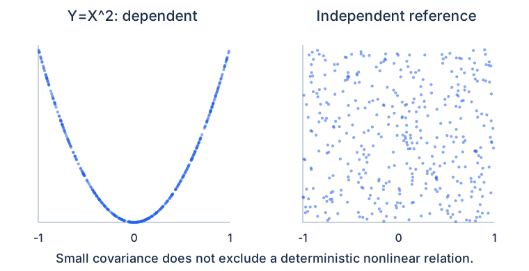
The CS counterpart has three equiprobable values and no integration prerequisite; AI learners additionally derive the continuous square relation with Module17. The script generates its actual scatter figure during the course build. Compare near-zero sample coefficients with the exact zero population covariance and the exactly satisfied nonlinear relation.
Lab3 · Variance faults and optional covariance geometry
Download lab3_variance_and_covariance_geometry.py
"""Repair an independence variance shortcut; optional AI covariance/PCA geometry."""
from fractions import Fraction as F
from math import sqrt

if __name__ == "__main__":
    p = F(3, 10)
    vx = p*(1-p)
    cov = vx  # Y=X, not an independent copy.
    correct = vx+vx+2*cov
    print("CS: X Bernoulli(.3), Y=X")
    print("Var(X)=%s Cov(X,Y)=%s Var(X+Y)=%s wrong independent sum=%s" % (
        vx, cov, correct, 2*vx))
    assert correct == F(21, 25)
    data = [(-2., -1.), (-1., -.5), (1., .5), (2., 1.)]
    n = len(data)
    mean = [sum(row[i] for row in data)/n for i in range(2)]
    centered = [[row[i]-mean[i] for i in range(2)] for row in data]
    covariance = [[sum(row[i]*row[j] for row in centered)/n for j in range(2)] for i in range(2)]
    principal, orthogonal = [2/sqrt(5), 1/sqrt(5)], [-1/sqrt(5), 2/sqrt(5)]
    print("AI geometry (Modules12/14): covariance uses denominator N, training mean only")
    print("mean:", mean, "covariance:", covariance)
    for name, direction, eigenvalue in (("principal", principal, 3.125), ("orthogonal", orthogonal, 0.)):
        scores = [sum(row[i]*direction[i] for i in range(2)) for row in centered]
        variance = sum(s*s for s in scores)/n
        matrix_product = [sum(covariance[i][j]*direction[j] for j in range(2)) for i in range(2)]
        assert max(abs(matrix_product[i]-eigenvalue*direction[i]) for i in range(2)) < 1e-12
        assert abs(variance-eigenvalue) < 1e-12
        print("%s direction=(%.6f,%.6f) projected variance=%.6f eigenvalue=%.6f" % (
            name, *direction, variance, eigenvalue))
    sample_covariance = [[v*n/(n-1) for v in row] for row in covariance]
    print("denominator N-1 covariance:", sample_covariance)
    print("Direction unchanged by common scaling; target covariance and estimator convention differ.")
    print("PASS: dependence contributes twice its covariance; PSD covariance can be singular")
CS: X Bernoulli(.3), Y=X
Var(X)=21/100 Cov(X,Y)=21/100 Var(X+Y)=21/25 wrong independent sum=21/50
AI geometry (Modules12/14): covariance uses denominator N, training mean only
mean: [0.0, 0.0] covariance: [[2.5, 1.25], [1.25, 0.625]]
principal direction=(0.894427,0.447214) projected variance=3.125000 eigenvalue=3.125000
orthogonal direction=(-0.447214,0.894427) projected variance=0.000000 eigenvalue=0.000000
denominator N-1 covariance: [[3.3333333333333335, 1.6666666666666667], [1.6666666666666667, 0.8333333333333334]]
Direction unchanged by common scaling; target covariance and estimator convention differ.
PASS: dependence contributes twice its covariance; PSD covariance can be singular
Repair the independence shortcut for Y=X. The optional AI section uses Modules12/14 to compare projected variance with eigenvalues and states its N denominator explicitly. Explain why changing to N−1 rescales the matrix without selecting a different direction in this example.
Fourteen exercises with full solutions
Exercises1–12 are required with equal-time branch alternatives. Optional Exercises13–14 add35 minutes beyond the ten-hour core schedule.
A search position has masses1:1/2,2:1/4,3:1/8,4:1/8. Compute expected comparisons and state what a uniform assumption changes.
Show solution
Weighted sum15/8=1.875, also tail sum1+1/2+1/4+1/8. Uniform position gives5/2. Worst successful cost4 is unchanged. A failed-search case must be separately modelled if present.
For X Bernoulli(.3), compute E[X²], variance, and variance of2X+5.
Show solution
X²=X, so E[X²]=.3. Var=.3−.09=.21. Affine variance4(.21)=.84; the shift5 changes only the mean.
For the lesson’s exact joint table, compute Cov(X,Y) and Var(X+Y).
Show solution
EX1/4,EY3/4,EXY1/4, so Cov1/16. Variances3/16 and15/16 give VarSum20/16=5/4. Dropping twice covariance incorrectly gives9/8.
For X equally likely−1,0,1 and Y=X², compute both means, covariance and one conditional demonstration of dependence.
Show solution
EX0,EY2/3,EXY0,Cov0. P(Y=0|X=0)=1 differs from P(Y=0)=1/3. Both variances are positive, so correlation0 is defined but does not imply independence.
Prove finite linearity of expectation without using independence and derive expected event count.
Show solution
Sum(aX+bY)p_ω over outcomes and distribute the finite sum to obtain aEX+bEY. For indicators E1_A=P(A), so EΣ1_Ai=ΣP(A_i), even when events overlap or depend. No joint product assumption appears.
Prove the variance-of-sum identity and identify the independence shortcut’s assumptions.
Show solution
Centre X,Y, expand(X_c+Y_c)², and average to obtain VX+VY+2Cov. Finite second moments ensure all terms exist. Independence gives E[XY]=EXEY and zero covariance, while uncorrelatedness alone also removes the cross term without establishing full independence.
Prove total variance using the conditional-mean residual and explain the cross term.
Show solution
Let m(Y)=E[X|Y]. Decompose X−EX=(X−m)+(m−EX). The squared residual’s expectation is EVar(X|Y); the mean-shift square is Var(m). Conditional averaging gives E[X−m|Y]=0, so the cross term vanishes. Finite variance and the correct marginal case weights are required.
In the joint table, calculate E[X|Y=0], E[X|Y=2] and their weighted total mean.
Show solution
Column masses5/8 and3/8 give means1/5 and1/3. Their weighted average1/8+1/8=1/4 matches EX. The equal average4/15 would correspond to a different mixture, not this Y distribution.
CS: Y=X for Bernoulli(.3); compute Var(X+Y). AI alternative: compute projected variances for the line-data covariance and its principal/perpendicular directions.
Show solution
CS: X+Y=2X, so variance4(.21)=.84, with covariance.21 supplying the missing cross terms. AI: aᵀCa is3.125 for(2,1)/√5 and0 for(−1,2)/√5, consistent with the exact line relation and PSD singularity.
Explain why E[X|Y] minimises squared prediction error among functions of Y, and what remains when a predictor is fitted from data.
Show solution
The expansion gives risk(a)=risk(m)+E[(m−a)²], because conditional residual orthogonality kills the cross term. Thus the true conditional mean is optimal up to null sets. A fitted estimate still needs sampling, approximation and evaluation assumptions; the population theorem does not certify its finite-data performance.
A symmetric square sample has small correlation and is declared independent; another report assigns correlation zero when X is constant. Repair both.
Show solution
The square relation determines Y from X despite zero population covariance; use its conditional distribution or relation residual to diagnose dependence. If X has zero variance, covariance is zero but correlation divides by zero and is undefined. A small sample coefficient alone is not an independence certificate.
A report averages conditional means equally despite unequal group masses and calls every PSD covariance invertible. Repair both.
Show solution
Total expectation weights conditional means by actual group probabilities. The lesson table uses5/8 and3/8, not equal weights. PSD only guarantees nonnegative projected variances; exact linear relations produce zero directions and a singular matrix. Invertibility needs positive definiteness.
CS: prove the squared-risk orthogonality expansion for a finite joint table. AI alternative: prove covariance transforms as AΣAᵀ and is PSD.
Show solution
CS: for each positive y, sum(X−m(y))p(x|y)=0; multiply by m(y)−a(y), then weight by p_Y(y) to kill the cross term. AI: Y−EY=A(X−μ), so expected outer products give AΣAᵀ. For every v, vᵀΣv=E[(vᵀ(X−μ))²]≥0.
CS: justify normalisation and infinite mean for masses1/[n(n+1)], then explain the symmetric signed mean. AI alternative: prove independence of Gaussian blocks with SPD block-diagonal covariance.
Show solution
CS: telescoping prefix1−1/(N+1)→1; meanΣ1/(n+1) diverges by powers-of-two blocks. Splitting signs gives both positive and negative expectations infinite, so the signed mean is undefined despite symmetric finite truncations. AI: inverse and determinant of block-diagonal Σ split by block, so its joint Gaussian density factors into marginal densities. The Gaussian joint assumption is essential.
Ten-question self-check
Show answer
X=1 mass1/4, Y=2 mass3/8, EX1/4,EY3/4,EXY1/4,Cov1/16; variances3/16,15/16 give VarSum5/4. Conditional means1/5,1/3 with masses5/8,3/8 average to1/4. Expected conditional variance11/60 plus variance of conditional mean1/240 equals3/16. Symmetric X with Y=X² is dependent despite covariance zero. All table moments are finite; sample coefficients fluctuate and do not establish the whole population law.
Reading with a purpose
Use expectation, joint distributions and conditioning in MIT 6.041SC, with covariance and Gaussian selections in the authors’ Mathematics for Machine Learning companion for the optional AI branch. The lesson gives complete elementary finite proofs and explicit continuous prerequisites.
| When | Selection and question |
|---|---|
| Session1 · 15 minutes | Expectation and moments: which operations need independence and which only integrability? |
| Session4 · 15 minutes | Conditional expectation and covariance: which information survives a low-order summary? |
Retrieval exit task and next step
Compute weighted costs and joint moments, prove linearity and variance identities, explain zero covariance with dependence, and derive total expectation/variance. AI learners additionally prove covariance PSD and qualified Gaussian factorisation, then connect empirical variance to centred PCA.
Exit task: reproduce the exact table’s variance decomposition3/16=11/60+1/240 and explain why its conditional means need5/8 and3/8 weights. Give a separate nonlinear uncorrelated-but-dependent example.
Ready to move on: you can attach averages and variation to explicit distributions and moment assumptions. Limit theorems and Monte Carlo next use these quantities to describe sample-mean behaviour with stated independence and uncertainty contracts. See the course overview.
Notation and bilingual terminology
| Term or notation | Meaning | 中文 |
|---|---|---|
| E[X] / E[ | X | ] |
| Var / σ | Centred second moment / standard deviation | 方差、标准差 |
| p(x,y) / marginal | Joint masses / summed retained-variable law | 联合、边缘分布 |
| Cov / ρ | Centred product moment / dimensionless correlation | 协方差、相关系数 |
| E[X | Y] / total variance | Conditional-mean variable / within-plus-between decomposition |
| Σ / PSD | Covariance matrix / nonnegative projected variance | 协方差矩阵、半正定 |
| Empirical distribution | Mass1/N per observed record | 经验分布 |